rcorex: Discover latent structure in high dimensional data.

Total correlation explanation is method for discovering latent structure in high dimensional data. Total correlation explanation has been implemented in Python as CorEx and related modules (https://github.com/gregversteeg/CorEx). The initial aim of rcorex is to implement Total Correlation Explanation in the R statistical software, specifically to replicate the functionality of the BioCorEx Python module ( https://github.com/gregversteeg/bio_corex ) which is designed to be suitable for biomedical datasets. This is implemented in the biocorex() command.

The theoretical framework behind the CorEx and Bio CorEx Python modules are laid out in the following academic papers:

Installation

rcorex can be installed from Github:

# install.packages("remotes")
remotes::install_github("jpkrooney/rcorex")

Minimal example

To fit a CorEx model in rcorex we can use the biocorex() command. biocorex() accepts a data.frame or a matrix as input, however as with the Python implementation of Bio CorEx, all variables must have the same data-type and currently only “discrete” or “gaussian” data are allowed as marginal descriptions, which apply to all columns.

library(rcorex)
# make a small dataset
df1 <- matrix(c(0,0,0,0,0,
             0,0,0,1,1,
             1,1,1,0,0,
             1,1,1,1,1), ncol=5, byrow = TRUE)

# fit biocorex
set.seed(1234)
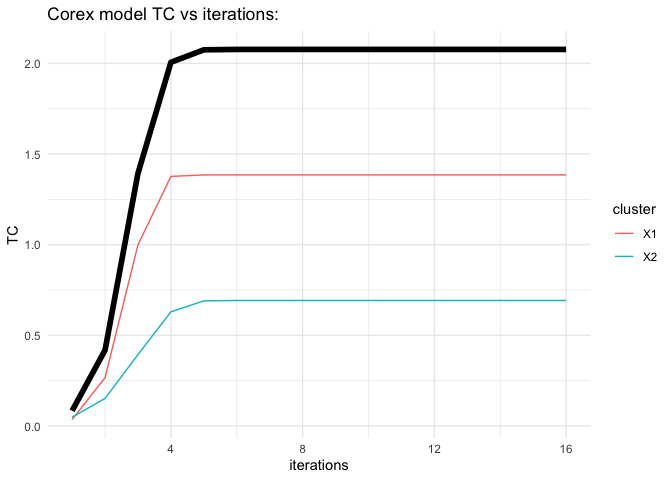
fit1 <- biocorex(df1, n_hidden = 2, dim_hidden = 2, marginal_description = "discrete", logpx_method = "pycorex")
#> Calculating single iteration of corex
plot(fit1)

summary(fit1)
#> rcorex model call: 
#> biocorex(data = df1, n_hidden = 2, dim_hidden = 2, marginal_description = "discrete", 
#>     logpx_method = "pycorex")
#> Data dimensions: 4 samples (rows) by 5 variables (columns).
#> Latent variable parameters: rcorex searched for 2 hidden variables with 2 possible states.
#> Model outcome state: Converged
#> Numer of iterations performed: 16
#> Total TCS at final iteration: 2.0769

# What was the total correlation for each hidden dimension ?
fit1$tcs
#> [1] 1.3847955 0.6921477

# Which variables were clustered together?
fit1$clusters
#> [1] 0 0 0 1 1

# Which labels were assigned to each row of data for hidden cluster 1?
fit1$labels[, 1]
#> [1] 1 1 0 0

# And for hidden cluster 2?
fit1$labels[, 2]
#> [1] 0 1 0 1

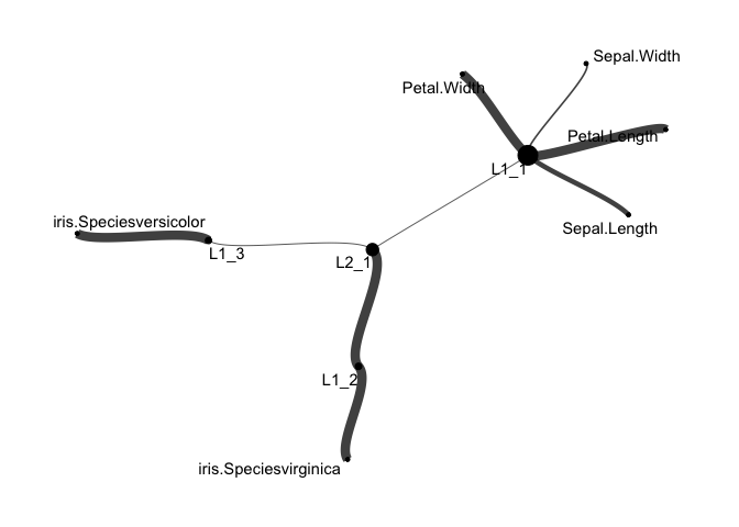
Hierarchical CorEx example

rcorex can search for hierarchical structure in data by using the labels output from an rcorex object as the input to the next layer in the hierarchy. This is shown in the following example using R’s inbuilt iris dataset.

library(rcorex)
library(ggraph)
#> Loading required package: ggplot2

set.seed(1234)

# Load iris dataset
data("iris")

# Need to convert species factor variable to indicator variables
iris <- data.frame(iris , model.matrix(~iris$Species)[,2:3])
iris$Species <- NULL

# fit first layer of CorEx 
layer1 <- biocorex(iris, 3, 2, marginal_description = "gaussian", repeats = 5, logpx_method = "pycorex")
#>  Calculating repeat # 1
#>  Calculating repeat # 2
#>  Calculating repeat # 3
#>  Calculating repeat # 4
#>  Calculating repeat # 5
#> 3 out of 5 repeat runs of biocorex converged.
#> Returning biocorex with highest TC of all converged runs - unconverged runs will not be included in comparison of runs.

Note the use of the repeats = 5 argument to biocorex. This acts to run biocorex not once, but 5 times and biocorex automatically selects the run which produces the maximal TC to return to the user (unless the return_all_runs argument is set to TRUE).

We can then use the labels from layer1 as the input for a second layer of CorEx to discover hierarchical structure. Note that the value used for n_hidden should be lower in the second layer than it was in the first.

# fit second layer of CorEx
layer2 <- biocorex(layer1$labels, 1,2, marginal_description = "discrete", repeats = 5, logpx_method = "pycorex")
#>  Calculating repeat # 1
#>  Calculating repeat # 2
#>  Calculating repeat # 3
#>  Calculating repeat # 4
#>  Calculating repeat # 5
#> 5 out of 5 repeat runs of biocorex converged.
#> Returning biocorex with highest TC of all converged runs - unconverged runs will not be included in comparison of runs.

# make a network tidygraph of hierarchical layers
g_hier <- make_corex_tidygraph( list(layer1, layer2))

# Plot network graph of hierarchical layers
ggraph(g_hier, layout = "fr") +
    geom_node_point(aes(size = node_size), show.legend = FALSE) +
    geom_edge_hive(aes(width = thickness), alpha = 0.75, show.legend = FALSE) +
    scale_edge_width(range = c(0.3, 3)) +
    geom_node_text(aes(label = names), repel = TRUE) +
    theme_graph()

Additional hierarchical layers can be identified in larger datasets.

Citation

If you find rcorex useful in academic work please cite the package as follows:

citation("rcorex")
#> 
#> To cite rcorex in publications use:
#> 
#>   Rooney JPK (2021). rcorex: Discover latent structure in high
#>   dimensional data. R package version 0.2.3.
#>   https://github.com/jpkrooney/rcorex. doi: 10.5281/zenodo.5235604.
#> 
#> A BibTeX entry for LaTeX users is
#> 
#>   @Manual{,
#>     title = {rcorex: Discover latent structure in high dimensional data.},
#>     author = {James PK Rooney},
#>     year = {2021},
#>     note = {R package version 0.2.3},
#>     doi = {10.5281/zenodo.5235604},
#>     url = {https://github.com/jpkrooney/rcorex},
#>   }