To get started: Fork this repository then issue
git clone --recursive http://github.com/[username]/geometry-processing-mesh-reconstruction.git
See introduction.
Once built, you can execute the assignment from inside the build/ using
./mesh-reconstruction [path to point cloud]
In this assignment, we will be implementing a simplified version of the method in "Poisson Surface Reconstruction" by Kazhdan et al. 2006. (Your first "task" will be to read and understand this paper).
Many scanning technologies output a set of
For shape analysis, visualization and other downstream geometry processing phases, we would like to convert this finitely sampled point cloud data into an explicit continuous surface representation: i.e., a triangle mesh (a special case of a polygon mesh).
Converting the point cloud directly to a triangle mesh makes it very difficult to ensure that the mesh meets certain topological postconditions: i.e., that it is manifold, closed, and has a small number of holes.
Instead we will first convert the point cloud sampling representation into a
an implicit surface
representation: where the
unknown surface is defined as the
level-set of some function
\[ ∂\S = {\x ∈ \R³ | g(\x) = σ}. \]
On the computer, it is straightforward
discretize an implicit
function. We define a regular 3D grid of
voxels containing at least the bounding
box of
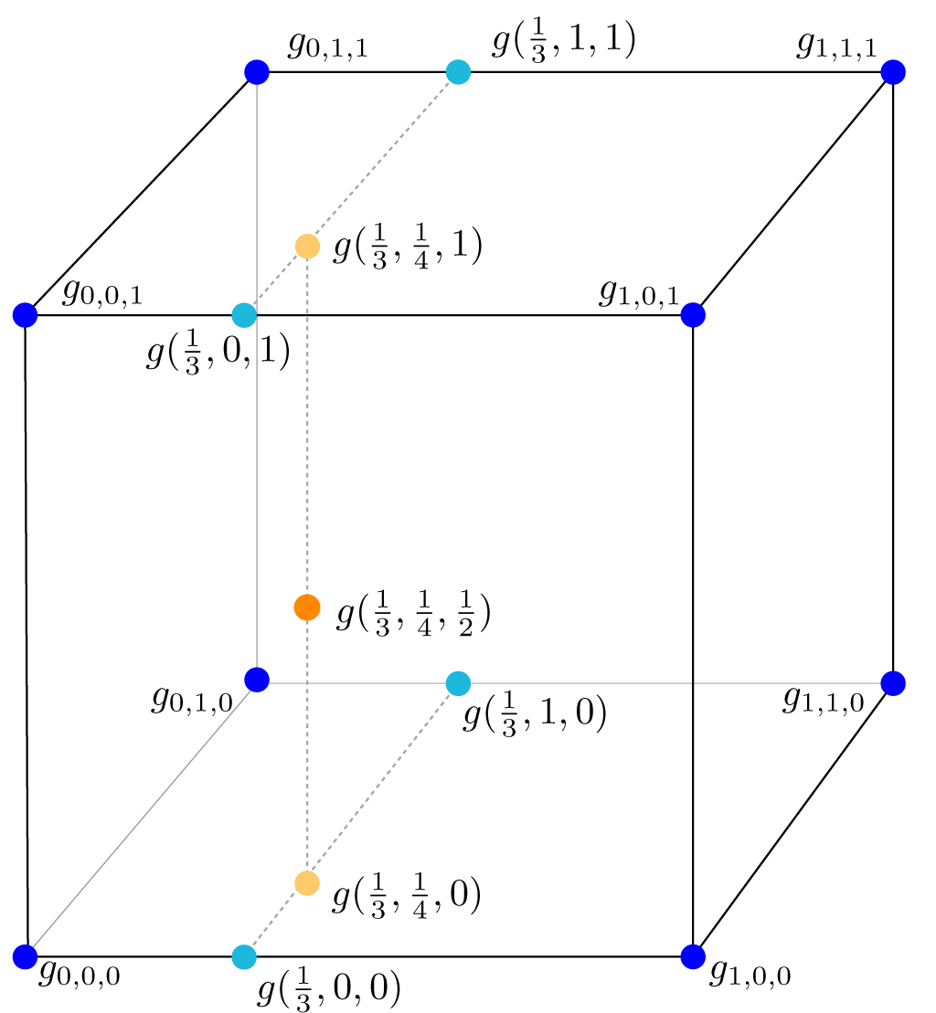
For example, consider a point
An implicit surface stored as the level-set of a trilinearly interpolated grid
can be contoured into a triangle mesh via the Marching Cubes
Algorithm.
For the purposes of this assignment, we will treat this as a black
box. Instead, we focus on
determining what values for
We assume that our set of points
\[ ∫\limits_\S 1 ;dA. %_ \]
We can rewrite this definite integral as an indefinite integral over all of
\[ ∫\limits_{\R³} χ_\S(\x) ;dA, \]
by introducing the characteristic
function of
\[
χ_\S(\x) = \begin{cases}
1 & \text{ if
Compared to typical implicit surface
functions, this function
represents the surface
One of the key observations made in [Kazhdan et al. 2006] is that the gradient of a infinitesimally mollified (smoothed) characteristic function:
- points in the direction of the normal near the surface
$∂\S$ , and - is zero everywhere else.
Our goal will be to use our points
- we know how to compute
$∇g$ at each node location$\x_{i,j,k}$ , and - our input points
$\P$ all lie perfectly at grid nodes:$∃\ \x_{i,j,k} = \p_ℓ$ .
We will find out these assumptions are not realistic and we will have to relax them (i.e., we will not make these assumptions in the completion of the tasks). However, it will make the following algorithmic description easier on the first pass.
If our points
\[ ∇g(\x_{i,j,k}) = \v_{i,j,k} := \begin{cases} \vphantom{\left(\begin{array}{c}0\0\0\end{array}\right)} \n_ℓ & \text{ if $∃\ \p_ℓ = \x_{i,j,k}$}, \ \left(\begin{array}{c} 0\ 0\ 0\end{array}\right) & \text{ otherwise}. \end{cases} \]
This is a vector-valued equation. The gradients, normals and zero-vectors are
three-dimensional (e.g.,
Since we only need a single number at each grid node (the value of
Like many geometry processing algorithms confronted with such an over determined, we will optimize for the solution that best minimizes the error of equation:
\[ ‖ ∇g(\x_{i,j,k}) - \v_{i,j,k}‖². \]
We will treat the error of each grid location equally by minimizing the sum over all grid locations:
\[ \min_\g ∑_i ∑_j ∑_k ½ ‖ ∇g(\x_{i,j,k}) - \v_{i,j,k}‖², \]
where
Part of the convenience of working on a regular grid is that we can use the
finite difference
method to approximate
the gradient
After revisiting our assumptions, we will be able to compute
approximations of
the
\[ \min_\g ½ ‖ \G \g - \v ‖², \]
or equivalently after expanding the norm:
\[ \min_\g ½ \g^\transpose \G^\transpose \G \g - \g^\transpose \G^\transpose \v + \text{constant}, \]
This is a quadratic "energy" function of the variables of
\[ \frac{∂}{∂\g} ½ \g^\transpose \G^\transpose \G \g - \g^\transpose \G^\transpose \v = 0. \]
Applying this derivative gives us a sparse system of linear equations
\[ \G^\transpose \G \g = \G^\transpose \v. \]
We will assume that we can solve this using a black box sparse solver.
Now, let's revisit our assumptions.
The gradient of a function
\[ ∇g(\x) = \left(\begin{array}{c} \frac{∂g(\x)}{∂x} \ \frac{∂g(\x)}{∂y} \ \frac{∂g(\x)}{∂z} \end{array}\right). \]
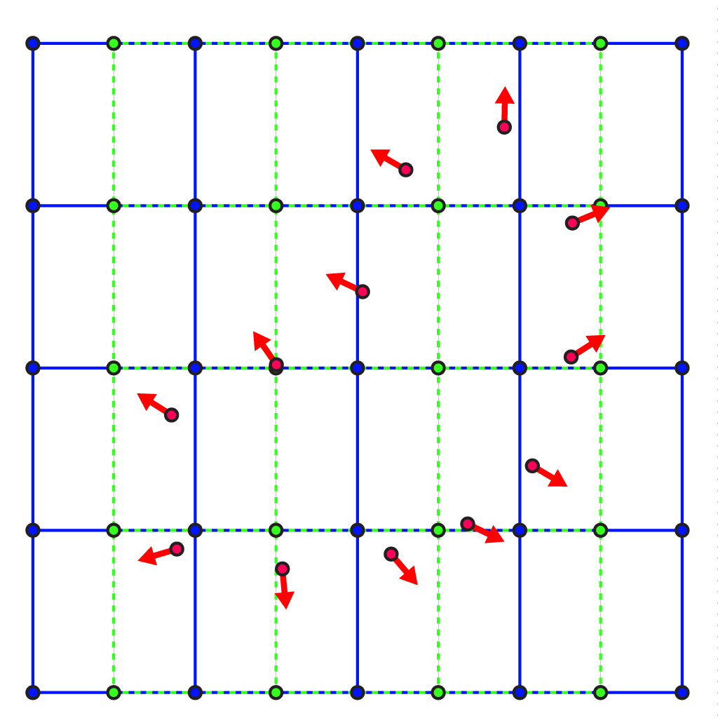
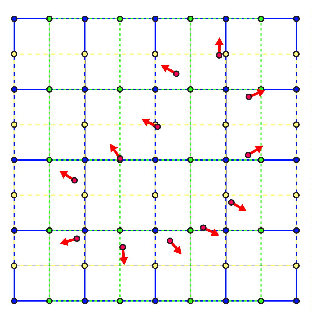
We will approximate each partial derivative individually. Let's consider the
partial derivative in the
The partial derivative in the
\[ \frac{∂g(\x_{i-½,j,k})}{∂x} = \frac{g_{i,j,k} - g_{i-1,j,k}}{h}, \]
where we use the index
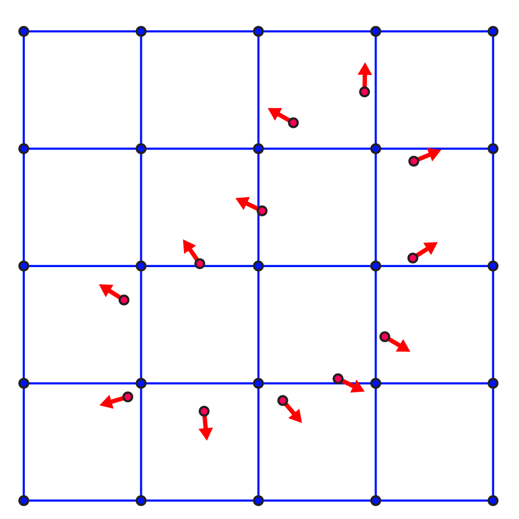
The following pictures show a 2D example, where
The partial derivatives of
The partial derivatives of
Letting
\[
\D^x_{i-½,j,k}(ℓ) =
\begin{cases}
-1 & \text{ if
Now, obviously in our code we cannot index the column vector
$\g$ by a triplet of numbers${i,j,k}$ or the rows of$\D^x$ by the triplet${i-½,j,k}$ . We will assume that$\g_{i,j,k}$ refers tog(i+j*n_x+k*n_y*n_x). Similarly, for the staggered grid subscripts${i-½,j,k}$ we will assume that$\D^x_{i-½,j,k}(ℓ)$ refers to the matrix entryDx(i+j*n_x+k*n_y*n_x,l), where the$i-½$ has been rounded down.
We can similarly build matrices
\[ \G = \left(\begin{array}{c} \D^x \ \D^y \ \D^z \end{array}\right) ∈ \R^{ \left((n_x-1)n_yn_z + n_x(n_y-1)n_z + n_xn_y(n_z-1)\right)×n_xn_yn_z} \]
This implies that our vector
\[ \v = \left(\begin{array}{c} \v^x \ \v^y \ \v^z \end{array}\right) ∈ \R^{ \left((n_x-1)n_yn_z + n_x(n_y-1)n_z + n_xn_y(n_z-1)\right)×1}. \]
This leads to addressing our second assumption.
At this point, we would actually liked to have had that our input normals
were given component-wise on the staggered grid. Then we could immediate stick
them into
To remedy this, we will distribute each component of each input normal
For example, consider the normal
\[ \x_{½,0,0}, \ \x_{1½,0,0}, \ \x_{½,1,0}, \ \x_{1½,1,0}, \ \x_{½,0,1}, \ \x_{1½,0,1}, \ \x_{½,1,1}, \text{ and } \ \x_{1½,1,1} \]
Each of these staggered grid nodes has a corresponding
We will distribute
\[
v^x_{½,0,0} = w_{ ½,0,0}\left(\x_{1,¼,½}\right)\ n_x, \
v^x_{1½,0,0} = w_{1½,0,0}\left(\x_{1,¼,½}\right)\ n_x, \
\vdots \
v^x_{1½,1,1} = w_{1½,1,1}\left(\x_{1,¼,½}\right)\ n_x.
\]
where
\[ n_x = \ w_{ ½,0,0}( \x_{1,¼,½} ) \ v^x_{ ½,0,0} + \ w_{1½,0,0}( \x_{1,¼,½} ) \ v^x_{1½,0,0} + \ \vdots \ w_{1½,1,1}( \x_{1,¼,½} )\ v^x_{1½,1,1}. \]
Since we need to do these for the
\[ ( \W^x \v^x ) ∈ \R^{n×1} \]
the transpose of
\[ \v^x = (\W^x)^\transpose \N^x. \]
Using this definition of
BTW, what's Poisson got to do with it?
The discrete energy minimization problem we've written looks like the squared norm of some gradients. An analogous energy in the smooth world is the Dirichlet energy:
\[ E(g) = ∫_Ω ‖∇g‖² dA \]
to minimize this energy with respect to
$g$ as an unknown function, we need to invoke Calculus of Variations and Green's First Identity. In doing so we find that minimizers will satisfy:\[ ∇⋅∇ g = 0 \text{ on Ω}, \]
known as Laplaces' Equation.
If we instead start with a slightly different energy:
\[ E(g) = ∫_Ω ‖∇g - V‖² dA, \]
where
$V$ is a vector-valued function. Then applying the same machinery we find that minimizers will satisfy:\[ ∇⋅∇ g = ∇⋅V \text{ on Ω}, \]
known as Poisson's equation.
Notice that if we interpret the transpose of our gradient matrix
$\G^\transpose$ as a divergence matrix (we can and we should), then the structure of these smooth energies and equations are directly preserved in our discrete energies and equations.This kind of structure preservation is a major criterion for judging discrete methods.
Constant functions have no gradient. This means that we can add a constant
function to our implicit function
\[ ∇g = ∇(g+c) = ∇g + ∇c = ∇g + 0. \]
The same is true for our discrete gradient matrix
This is potentially problematic for our least squares solve: there are many
solutions, since we can just add a constant. Fortunately, we don't really
care. It's elegant to say that our surface is defined at
To this end we just need to find a solution
As suggested in [Kazhdan et al. 2006], we can pick a good iso-value by
interpolating our solution
\[ σ = \frac{1}{n} \mathbf{1}^\transpose \W \g, \]
where
Besides the insights above, a major contribution of [Kazhdan et al. 2006] was to setup and solve this problem on an adaptive grid rather than a regular grid. They also track "confidence" of their input data effecting how they smooth and interpolate values. As a result, their method is one of the most highly used surface reconstruction techniques to this day.
Consider adding your own insights to the wikipedia entry for this method.
This reading task is not directly graded, but it's expected that you read and understand this paper before moving on to the other tasks.
Given a regular finite-difference grid described by the number of nodes on each
side (nx, ny and nz), the grid spacing (h), and the location of the
bottom-left-front-most corner node (corner), and a list of points (P),
construct a sparse matrix W of trilinear interpolation weights so that `P = W
- x`.
Given a regular finite-difference grid described by the number of nodes on each
side (nx, ny and nz), the grid spacing (h), and a desired direction,
construct a sparse matrix D to compute first partial derivatives in the given
direction onto the staggered grid in that direction.
Given a regular finite-difference grid described by the number of nodes on each
side (nx, ny and nz), and the grid spacing (h), construct a sparse
matrix G to compute gradients with each component on its respective staggered
grid.
then simply concatenate these together to make
G.
Given a list of points P and the list of corresponding normals N, construct
a implicit function g over a regular grid (built for you) using approach
described above.
You will need to distribute the given normals N onto the staggered grid
values in v via sparse trilinear interpolation matrices Wx, Wy and Wz
for each staggered grid.
Then you will need to construct and solve the linear system
Determine the iso-level sigma to extract from the g.
Feed this implicit function g to igl::copyleft::marching_cubes to contour
this function into a triangle mesh V and F.
Make use of fd_interpolate and fd_grad.
Eigen has many different sparse matrix solvers. For these very regular matrices, it seems that the conjugate gradient method will outperform direct methods such as Cholesky factorization. Try
Eigen::BiCGSTAB.
Debug in debug mode with assertions enabled. For Unix users on the command line use:
cmake -DCMAKE_BUILD_TYPE=Debug ../but then try out your code in release mode for much better performance
cmake -DCMAKE_BUILD_TYPE=Release ../


