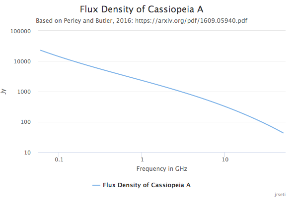
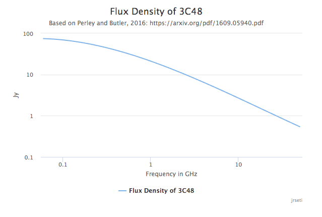
Calculates the flux densities of 20 sources as described in Perley and Butler, 2016: https://arxiv.org/pdf/1609.05940.pdf
This code basically uses the coefficients defined in Perley and Butler's paper and performs the following to calculate the flux. Note that νG is the frequency in GHz.
log(S) = a0 + a1 log(νG) + a2[log(νG)]2 + a3[log(νG)]3 + · · ·
It is important to note that the coefficients a0..a(n) as defined in the Perley and Butler paper are each a range of values such as 1.0440 ± 0.0010. The center value of each coefficient is used for these calculations, ignoring there is a range.
The decline in flux density over time is not taken into account for these calculations. Cassiopeia A, for example, is declining at a rate of approx 0.4%/year!
This project is also an exercise in creating a data set and also displaying the data as an interactive graph, automatically popping up a new page in the user's default browser.
Note that the graph is interactive and you can mouse over a data point and view the exact values in a tooltip.
Highcharts (https://www.highcharts.com/) is used to create the graph.
The following sources can be specified:
- J0133-3629
- 3C48
- Fornax A
- 3C123
- J0444-2809
- 3C138
- Pictor A
- Taurus A
- 3C147
- 3C196
- Hydra A
- Virgo A
- 3C286
- 3C295
- Hercules A
- 3C353
- 3C380
- Cygnus A
- 3C444
- Cassiopeia A
3c48: 12.077 Jy @ 2.000 GHz
This interactive graph should pop up in your browser:

