- Motivation/Hypothesis
- Dataset
- Models Used
- Computational Resources
- Training Models
- Transfer Learning
- Models Comparison
- Validation With Our Own Images
- Validation With Youtube Videos
- Conclusion And Future Work
- How To Run
- References
- Contributors
Our project aims to advance the field of autonomous driving through improved computer vision techniques. We hypothesize that by integrating state-of-the-art models for lane detection and object recognition, we can enhance the accuracy and reliability of self-driving systems.
We use BDD100K Dataset, which contains 100.000 images of diverse road scenes. This dataset is crucial for our project due to its comprehensive coverage of various driving conditions and high-quality annotations. Download
The BDD100K dataset is the largest driving video dataset with 100K videos and 10 tasks to evaluate the exciting progress of image recognition algorithms on autonomous driving.
- Number of Images: 100,000
- Resolution: 1280x720 pixels
- Annotations: Multiple types including object detection, lane marking, drivable area, and segmentation.
- Driving Conditions: Diverse, covering different weather conditions, times of day, and various locations.
- Object Detection: Bounding boxes for objects such as cars, pedestrians, traffic signs, and cyclists.
- Lane Marking: Polylines indicating the position of lane markings on the road.
- Drivable Area: Segmentation maps identifying areas that are drivable.
- Semantic Segmentation: Pixel-level labels for different objects and regions in the image.
- Instance Segmentation: Pixel-level labels with instance information for objects.
In order to train the LaneNet model with the BDD100K dataset, we have to previously transform it with the same transformation that the LaneNet model uses to be trained with the Original dataset, tuSimple.
- src/preprocessing/bdd100k_transform.py
The provided codeis used to generate training dataset masks for the BDD100K dataset, specifically for lane detection. It processes the dataset annotations and creates binary and instance masks for each image. The masks are used to train models for tasks such as semantic segmentation and lane detection in autonomous driving applications.\
LaneNet is our primary model for lane detection. It is a convolutional neural network (CNN) model designed specifically for lane detection in autonomous driving applications, which is crucial for tasks such as lane keeping, lane changing, and overall vehicle navigation. It employs a segmentation-based approach to identify and classify lane markings accurately.
LaneNet employs an encoder-decoder architecture to process input images and generate lane detection results. The encoder extracts high-level features from the input image using a series of convolutional layers, while the decoder reconstructs the spatial details to produce pixel-wise lane markings.
LaneNet uses a semantic segmentation approach combined with instance segmentation. The model segments the image into lane and non-lane regions and differentiates between individual lane markings. This dual approach allows LaneNet to handle multiple lanes simultaneously and distinguish between them.
A key feature of LaneNet is its use of embedding vectors. For each pixel classified as a lane, the network assigns an embedding vector that helps cluster pixels belonging to the same lane. This clustering is achieved through a discriminative loss function that encourages pixels of the same lane to have similar embeddings while separating different lanes.
For the LaneNet model, we use the ENet backbone. We train with the complete model, but for inference, we use only the head of the binary mask. The instance mask is not used to infer the final image.
LaneNet employs two primary loss functions:
- Binary Cross-Entropy Loss: Used in the segmentation branch to classify each pixel as lane or background. This loss helps the model learn to distinguish lane markings from the rest of the image.
- Discriminative Loss: Applied in the embedding branch to ensure that pixels belonging to the same lane are close together in the embedding space while being distinct from other lanes. It consists of three components:
- Variance Loss: Encourages embeddings within the same lane to be close to their mean.
- Distance Loss: Ensures that the means of different lanes are far apart.
- Regularization Loss: Aims to keep the embeddings small to avoid large values. By combining these loss functions, LaneNet can accurately segment lanes and differentiate between multiple lane markings, providing robust lane detection capabilities for autonomous driving applications.
This model is designed to perform lane detection using a combination of convolutional neural network (CNN) layers, feature pyramid networks (FPN), region of interest (RoI) alignment, and semantic segmentation heads.
This component is a convolutional neural network that extracts feature maps from input images. It uses:
- Several convolutional layers
- Batch normalization
- ReLU activations
The feature maps are extracted through a series of layers.
The FPN creates feature pyramids from the backbone's output. It:
- Combines feature maps from different levels (layers)
- Builds multi-scale feature maps
- Useful for detecting objects at various scales
This module aligns Regions of Interest (RoIs) of different sizes to a fixed size using feature maps from the FPN. It:
- Uses the spatial scale of the feature maps to properly resize and align the RoIs
- Distributes RoIs to different levels of the pyramid based on their size
This head performs semantic segmentation for lane detection. It consists of:
- Multiple convolutional layers
- A deconvolutional (upsampling) layer
- A final convolutional layer to produce the segmentation mask logits
This is the complete model that integrates all the components. It:
- Takes images and RoIs as input
- Processes them through the backbone, FPN, RoI align, and the semantic lane head
- Produces the final lane detection mask logits
The model uses Binary Cross-Entropy with Logits as the loss function for both training and evaluation:
F.binary_cross_entropy_with_logits(output, masks)This loss function combines a Sigmoid layer and the Binary Cross-Entropy loss in a single function. It's numerically stable and especially useful for tasks like lane detection where the output is a binary mask.
Key Features:
Automatically applies the sigmoid activation function to the model output before calculating the loss.
Provides better numerical stability than using a plain Sigmoid followed by Binary Cross-Entropy loss.
The primary evaluation metric used is Binary Accuracy:
acc = binary_accuracy(output, masks, threshold=0.5)This metric computes the accuracy of binary predictions:
It applies a threshold (default 0.5) to the model's output to create binary predictions. It then compares these binary predictions to the ground truth masks. The result is the proportion of correct predictions (both true positives and true negatives) among the total number of cases examined.
Key Points:
- Threshold: A value of 0.5 is used to convert the model's probabilistic output into binary predictions.
- Interpretation: An accuracy of 1.0 means perfect prediction, while 0.5 would be equivalent to random guessing for a balanced dataset.
Faster R-CNN is a two-stage object detection algorithm:
- Scans the image and proposes potential object regions
- Uses anchor boxes of various sizes and aspect ratios
- Outputs "objectness" scores and rough bounding box coordinates
- Takes proposed regions from RPN
- Performs classification (what object is it?)
- Refines bounding box coordinates
ResNet50 is a deep convolutional neural network with 50 layers:
- Uses residual connections (skip connections)
- Allows training of very deep networks by addressing vanishing gradient problem
- Composed of repetitive blocks:
- Convolutional layers
- Batch normalization
- ReLU activation functions
FPN enhances feature extraction:
- Creates a multi-scale feature pyramid
- Top-down pathway: Upsamples spatially coarser, but semantically stronger features
- Lateral connections: Merges features from the bottom-up and top-down pathways
- Helps detect objects across a wide range of scales
- COCO (Common Objects in Context) dataset:
- 330K images
- 1.5 million object instances
- 80 object categories
- Pre-training on COCO provides a strong starting point for transfer learning
The Faster R-CNN model typically uses a multi-task loss function that combines several components:
1. Classification Loss
- Type: Cross-Entropy Loss
- Purpose: Measures the error in classifying the object (e.g., car or truck)
- Applied to: Both the Region Proposal Network (RPN) and the final classifier
2. Bounding Box Regression Loss
- Type: Smooth L1 Loss (also known as Huber Loss)
- Purpose: Measures the error in predicting the bounding box coordinates
- Applied to: Both the RPN and the final regressor
- Advantage: Less sensitive to outliers compared to standard L2 loss
3. Objectness Loss
- Type: Binary Cross-Entropy Loss
- Purpose: Measures the error in predicting whether a region contains an object or not
- Applied to: RPN
The total loss is a weighted sum of these components:
Where:
- L_cls: Classification loss
- L_box: Bounding box regression loss
- L_rpn_cls: RPN classification loss (objectness)
- L_rpn_box: RPN bounding box regression loss
- λ: Balancing parameters for each loss component
The code uses two primary metrics for evaluation: Accuracy and Validation Loss. These are calculated in the evaluate_model function.
The accuracy metric in this implementation is based on the Intersection over Union (IoU) between predicted and ground truth bounding boxes.
-
For each image in the validation set:
- Compare each ground truth box with all predicted boxes
- Calculate IoU for each pair
- A prediction is considered correct if its IoU with a ground truth box exceeds a threshold (not explicitly defined in the code, typically 0.5)
-
Accuracy is then calculated as: Accuracy = Number of Correct Predictions / Total Number of Ground Truth Boxes
- Hardware: Personal Computer (PC)
- Processing Units:
- GPU (1): NVIDIA GeForce RTX 3080
- CPU (1): Intel® Core™ i9-12900K
- Training Duration: 87 hours
Our custom Lane Net model leveraged both CPU and GPU processing power on a personal computer. This configuration allows for faster training times compared to CPU-only setups, making it suitable for iterative development and experimentation.
- Hardware: Laptop
- Processing Unit: Single CPU
- Training Duration: 64 hours
The Mask R-CNN model, known for its effectiveness in instance segmentation tasks, was trained on a standard laptop configuration. This setup demonstrates the model's ability to be trained on consumer-grade hardware, albeit with a significant time investment.
- Platform: Google Cloud
- Processing Units:
- GPUs (2)
- CPU (4)
The Faster R-CNN model was trained using cloud computing resources, specifically on Google Cloud. This high-performance setup with multiple GPUs is ideal for training complex models or working with large datasets, significantly reducing training time compared to local machine setups. This model has been trained using 4 CPUs because we have a configuration with 4 workers in common. If we use fewer CPUs, the model's performance may degrade significantly, leading to potential bottlenecks and inefficiencies.
Training the three models is a long process requiring if it is possible use at least one gpu.
The source code is prepared to use tensorboard for analysis.
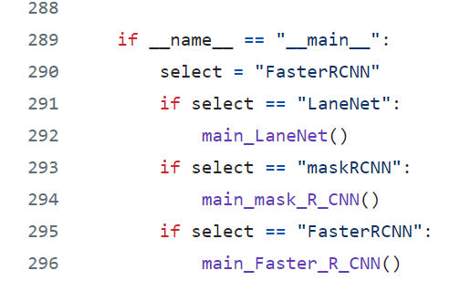
Every model must be trained separetly by choosing the righ one in the main as follows:\
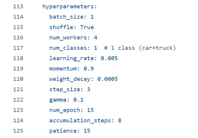
From the "configs/config.yaml" the training parameters are available. There the Hyperparameters con be configured. An example of the used parameters is the following:
After the training, the model parametrization file, will be created in the models folder. Use this file for any simulation.
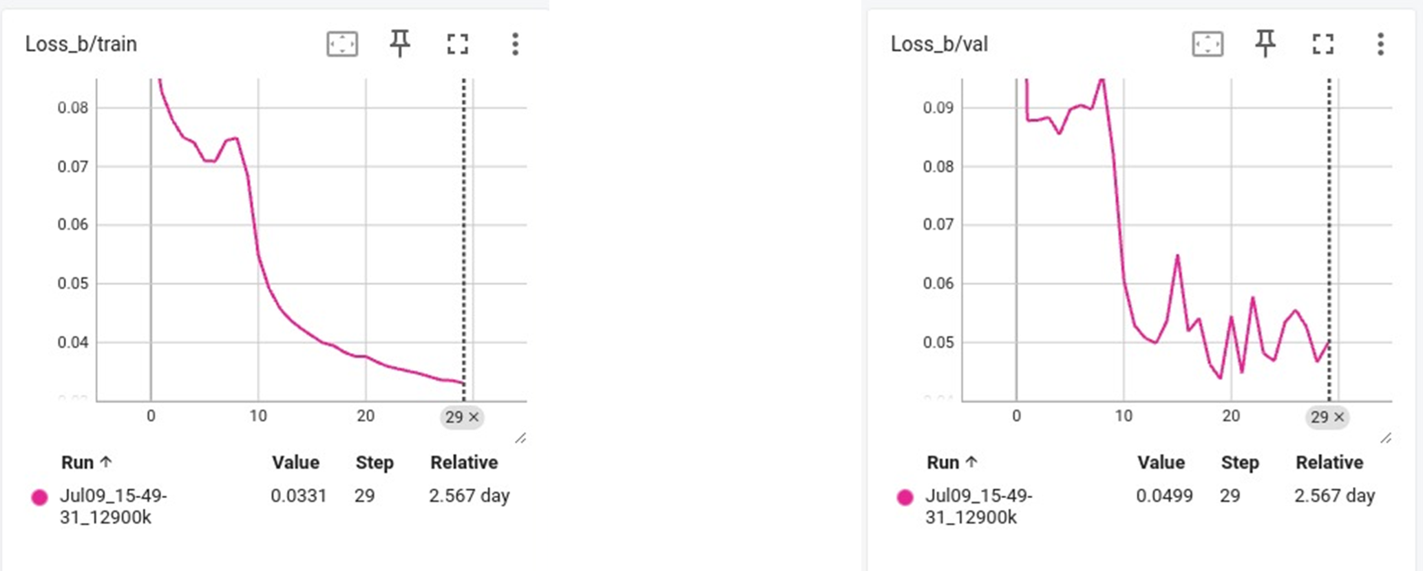
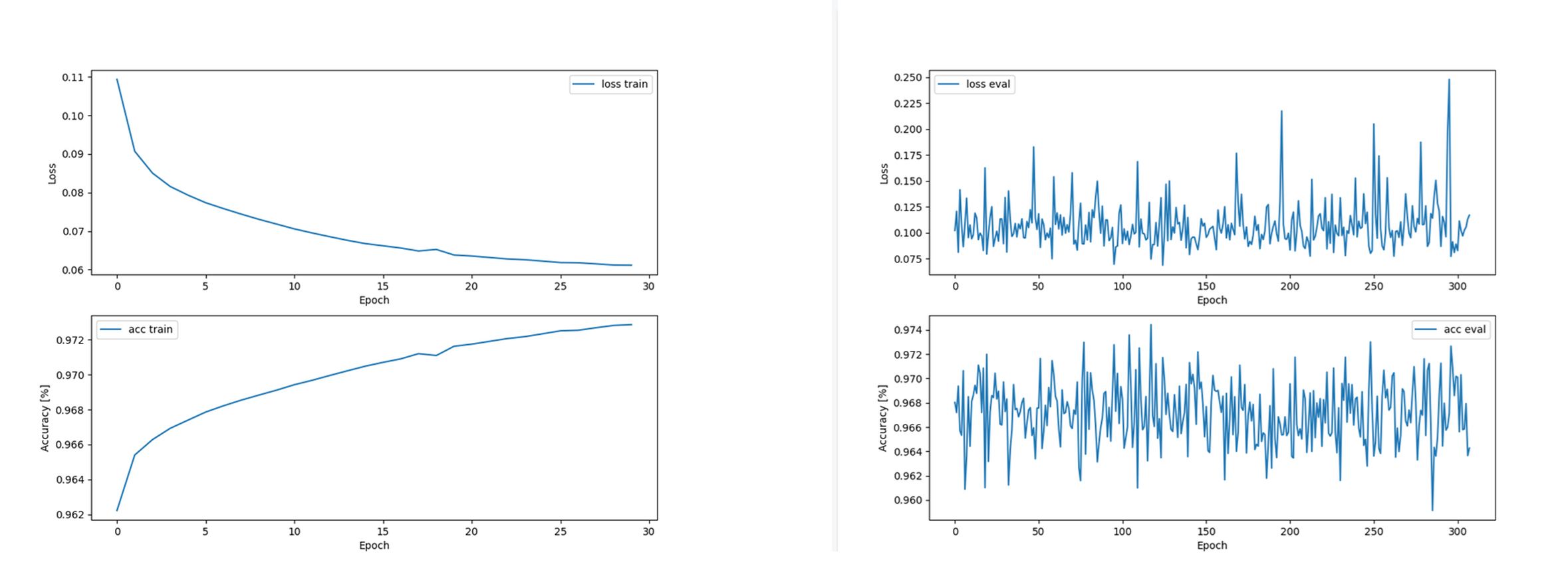
Some examples we get of loss/accuracy are show below:
Transfer learning is a machine learning method where a model developed for a task is reused as the starting point for a model on a second task.
The aim of our experiment was to check with a line detection model and an object detection model on a simple camera, we were able to predict on the road the direction that a self-driving system should follow, with proximity indicators of other vehicles.
To achieve this goal we decided to implement from scratch a LaneNET model and Mask R-CNN model, compare the results and apply the best one.
In addition we tried to implement a Faster R-CNN for object detection, to indicate other vehicles proximity.
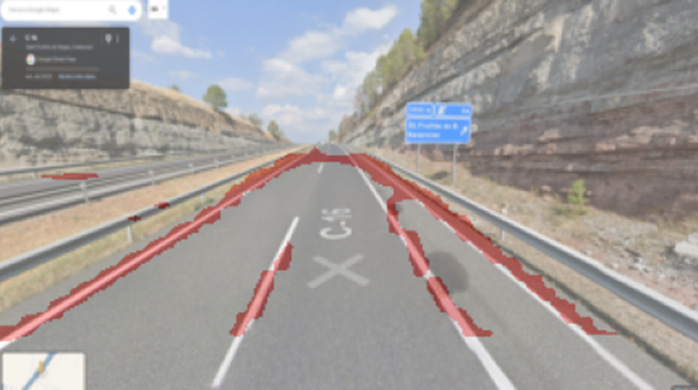
The first goal was get the lines detection, using two different sizes of image on the Mask R-CNN model devellopped from scratch (180x320 vs 480x854). The model was giving a small output of fixed dimension, causing that recover the original image size was only possible using the 180x320 size input.
We stop the trials due to the long train process (at this point we were training using a laptop with CPU).
The results using a google maps image as reference were as follows:
At the same time we were preparing the second model LaneNET to get a different performance. In this case we train the model focus on images of 480x854, expecting get a better precision. The model was get from the original paper and also using the original dataset (tuSimpleDataset).
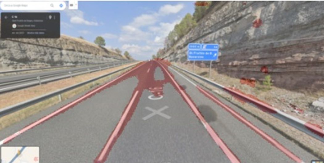 Figure2: LaneNET trained with tuSimpleDataset
The results were good, but not as good as we expected. At this point we decided adapt the bdd100k Dataset to the model to train it with a lot more samples. The result was surprising, a lot more of precision, just detecting the road lines.
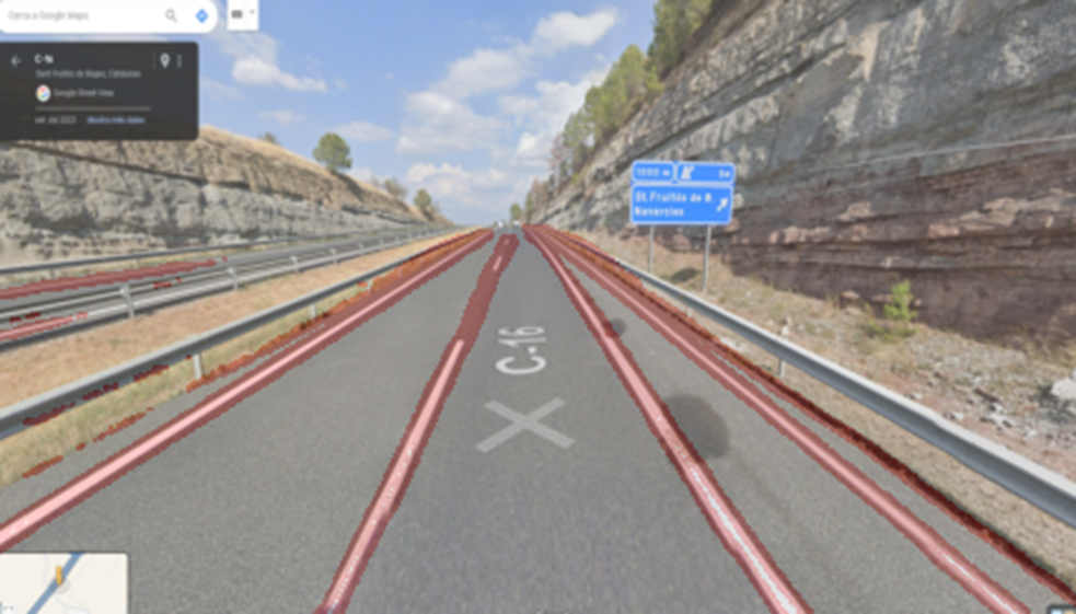 Figure3: LaneNET trained with bdd100k dataset
The next step was implement both models in a real video to validate real-world performance. It was done using a mobile in a car, driving on the highway.
The LaneNet model (right side) was a lot better than the Mask R-CNN (left side), like we expected. the surprising was that both models were able to detect the lines.
To achieve our goal we had some troubles like:
- The images size applied on the model had to match with the trained images size to get good results.
- The images focus had to be consistent with train dataset (landscape vs road).
- Difficult define the threshold to decide if it is point or not, it depends a lot of the image quality and resolution.
Once developed the line detection models, we create a simple algorithm to calculate the angle deviation from previous to current frame on a video, and we applied an addition calculation to rotate a possible wheeldrive. Basically, we tried to simulate a possible self-driving system.
This algorithm was based in the following steps:
- Find the center of the binary mask image.
- Calculate the image rotation from this point respect the previous image.
- Apply a simple calculation: angle_new = angle_old + (2 x angle_diff)
To give consistence to the experiment, we applied also the algorithm to the original image (left side). The results were as we expected, better on the LaneNET predictor (right side), than in the Mask R-CNN (center). The precision of the image, helped a lot to get a good response.
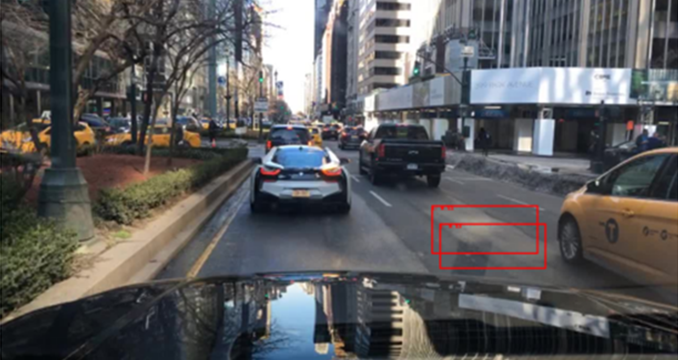
The last experiment was add an object detection to our system. We implent a Faster R-CNN from ResNet50 and what had to be simple, was complicated. We used a annotations from the same dataset bdd100k.
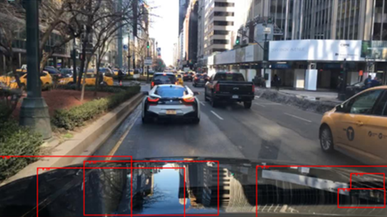
The training of this model required a lot of performance, so we started just when we get the option of train using a Google Cloud with GPU. We train for first time using 20000 images with 30 epochs, just looking for cars. The results were not like expected, were bad and not repetitive.
The train and validate loss didn’t go according, accuracy really bad and overfitting.
We increase the number of samples using less epochs and fixed the seed to be more deterministic. Also we include in out annotations the trucks.
The next train was also done using a GPU on Google Cloud, with 70000 samples and only 4 epochs, but the results still bad.
Train and validation loss graphs didn't go according and accuraccy was really bad.
Found that annotations were not properly scaled according to the image resize transform, so we tried to fix it and train it again, bu we expend the rest of Google Cloud balance we had. We couldn’t finish the tranning (we tried using local CPU but was too long), so we decided implement the pre-trained model.
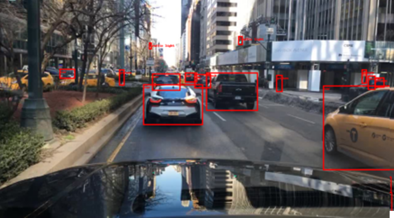
The results were satisfactory.
The final experiment was implement in the self-driving system the object detection and show the proximity of a car by colors:
- green, the vehicle was far
- yellow, the vehicle was close
- red, the vehicle was too close
To decide the color, we use the lower height of the box predicted. The results are visible in the following video.
The experiment was a success.
| LaneNet | FasterRCNN Object Detection | MaskRCNN Segmentation |
|---|---|---|
 |
 |
 |
Our project demonstrates how complicate is develop, debug and apply a model from scratch. We confirm how important is start from verified models and if it is possible pre-trained models to save time and resources for training. On the other side, we observe how from the theory, a model can be created from scratch and also works. A future work could focus on improve the models performance to be applied faster in real time, add new inputs additionally to a camera and develop a more sophisticated algorithms for self-driving.
- Clone repository
git clone https://github.com/jsabahu/AIDL24_SelfDriving.git
- Create a conda environment
conda create --name AIDL24_SelfDriving python=3.11.9
- Activate conda environment
conda activate AIDL24_SelfDriving
- Install requirements packages
pip install -r requirements.txt
- Download Dataset
https://dl.cv.ethz.ch/bdd100k/data/
- Transform data
python bdd100k_transform.py --src_dir path/to/bdd100k --val True --test True- LaneNet: Real-Time Lane Detection Networks for Autonomous Driving
- Towards End-to-End Lane Detection: an Instance Segmentation Approach
- LaneNet Lane Detection with Pytorch
- Faster R-CNN: Towards Real-Time Object Detection with Region Proposal Networks
- Mask R-CNN
- BDD100K Dataset: A Diverse Driving Video Dataset with Scalable Annotation Tooling
- ENet: A Deep Neural Network Architecture for Real-Time Semantic Segmentation
- Instance Segmentation by Jointly Optimizing Spatial Embeddings and Clustering Bandwidth
- Feature Pyramid Networks for Object Detection
- ImageNet Large Scale Visual Recognition Challenge
- Jordi Sabates
- Marc Ramon
- Marc Giné
- Fermin Gomila
Advisor: Daniel Fojo
Code:
Training:
