This package provides tools to analyze scientific research data, with a focus on plotting and statistical analysis. It is written in Python and was tested on Linux and MacOS.
This package was developed with Python 3.6 and was tested on Linux and MacOS 13. It depends on the following libraries (the version of the library on which I tested easy-data-analysis is shown between parentheses):
- matplotlib (3.1.3)
- numpy (1.18.4)
- pandas (0.25.3)
- pyyaml (5.3)
- scipy (1.4.1)
- sympy (1.5.1)
If you are new to installation of Python and its packages, a tutorial is on the Python's website.
Installing Python libraries is most easily done with pip3, simply run in a terminal:
pip3 install --upgrade <library>
easy-data-analysis is packaged and available through PyPI, you can install it by running in a terminal:
pip3 install --upgrade easy-data-analysis
Source distributions are also available here on GitHub, download the source and install it by running:
pip3 install <path>
easy-data-analysis is accessible through a command line interface which follows this syntax:
eda <command> <subcommand> [arguments ...]
Type this in your terminal for more information:
eda --help
eda configure <subcommand>
configure manages the default arguments of all commands, i.e. the behaviour of commands when you do not provide optional arguments.
Available subcommands:
spectrum: configureeda plot spectrumkinetics: configureeda plot kineticsdefault: rollback to the original configuration (the one provided when you install this package)
When you enter the configuration mode, instructions will be displayed before you are prompted for input. The name of the parameter is displayed followed by its current value between ( parentheses ). You have three possible actions (validate any of them by pressing <Enter>):
- keep the current value: leave the input field empty
- modify the current value: type your input (if a list is expected, use space to separate values)
- enter a void value (no value): enter 'none' (without quotes)
eda plot <subcommand> [arguments ...]
plot reads a CSV file and plots the data according to one of the following subcommands:
spectrumkinetics
This subcommand plots absorption spectra.
eda plot spectrum [arguments ...]
File names are positional arguments, they should be passed before optional argument. Optional arguments include:
-lor--labellabels for the plot legend--figure-sizewidth and height in inches--xcolumnname of the column containing x-axis values--ycolumnname of the column containing y-axis values--xlabellabel on the x-axis--ylabellabel on the y-axis--xlimitleft and right values for x-axis limits--ylimitbottom and top values for y-axis limits--skip-headernumber of rows to skip at the beginning of the file--legend-locationruneda plot spectrum -hfor more information--titletitle of the plot
For example:
eda plot spectrum file1.csv file2.csv -l experiment1 experiment2
For more information:
eda plot spectrum -h
This subcommand plots absorption kinetics curves. It can also plot an exponential model curve fitted on the data. Parameters of the model will be printed on the console.
eda plot kinetics [arguments ...]
File names are positional arguments and should be passed before optional arguments. Optional arguments include:
-lor--labellabels for the plot legend-for--fitfit the data with a mathematical model-mor--modelspecify the mathematical model used to fit the data. Choices include:exp(default) fit both first-order and second-order exponential models and selects the bestexp1fit a first-order exponentialexp2fit a second-order exponentiallinearfit a linear model
--init-paramsprovide initial parameters for the curve-fitting algorithm--skip-headernumber of rows to skip at the beginning of the file--xcolumnname of the column containing x-axis values--ycolumnname of the column containing y-axis values--xlabellabel on the x-axis--ylabellabel on the y-axis--xlimitleft and right values for x-axis limits--ylimitbottom and top values for y-axis limits--figure-sizewidth and height in inches--legend-locationruneda plot spectrum -hfor more information--titletitle of the plot
For example:
eda plot kinetics file1.csv file2.csv -l experiment1 experiment2 -f
For more information:
eda plot kinetics -h
You should do these two steps prior to the tutorial:
- install the
easy-data-analysispackage - download the CSV data files from
eda/docs/samples
These tutorials assume you have the default configuration. If you're not sure which configuration you have, run eda configure default.
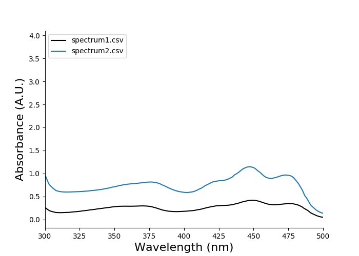
Plotting spectra is done by providing the file names to eda plot spectrum:
eda plot spectrum spectrum1.csv spectrum2.csv
You should see this output:
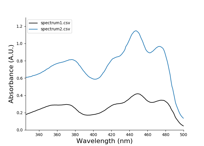
There is some empty space above the curves, because the data shows high absorbance below 300 nm but the plot does not display this by default. We can easily adjust the axes limits using the optional arguments --xlimit and --ylimit. These arguments both accept two values: the lower value and the higher value.
eda plot spectrum spectrum1.csv spectrum2.csv --xlimit 325 500 --ylimit 0 1.3
You should then see the following plot:
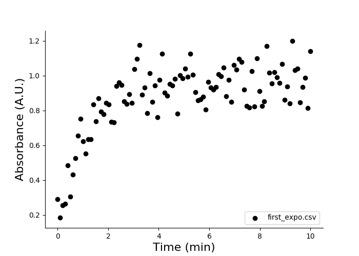
Plotting a kinetics curve is done by providing the file names(s) to eda plot kinetics:
eda plot kinetics first_expo.csv
You should see this output:
You do not need to provide optional arguments because the format of first_order.csv matches the default configuration. Files with various formats can be dealt with by changing or reviewing the configuration by running eda configure kinetics or by providing arguments to eda plot kinetics.
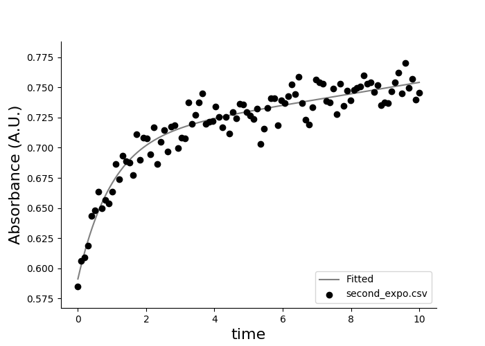
Let's plot and fit second_expo.csv. This file contains no rows to be skipped (the first line contains column names).
eda plot kinetics second_expo.csv -f -m exp2 --xcolumn time --ycolumn absorbance --xlabel time --skip-header 0
You should see this output:
When fitting a curve you will be provided with fitting results:
second_expo.csv
y = a1 * exp(k1 * x) + a2 * exp(k2 * x)
------------------------------
Parameter      Value   Std Err
------------------------------
a1           -0.1169    0.0069
a2           +0.7081    0.0051
k1           -1.0201    0.1330
k2           +0.0063    0.0010
R-square     0.91967
t1 (sec)       40.77
t2 (sec)     6600.02
The first line is the file name, the second line is the equation of the data model. The following lines show the value and standard error of the parameters of the equation. The R-square value indicates the goodness of fit and varies from 0 (poor fit) to 1 (perfect fit). The parameters t1 and t2 are the doubling times (or halving times for exponential decay) of the first and second components of the equation. They are calculated as:
t1 and t2 are shown in seconds and assume that you provide data in minute by default. If the time unit of your data is second, you can specify it by running eda configure kinetics and modify the parameter time_unit or by using the parameter --time-unit when calling eda plot kinetics.
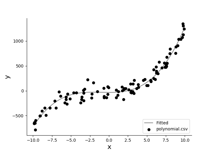
You may feel limited by the fitting models hard-coded in easy-data-analysis by default. You can provide your own mathematical equation when fitting a kinetics curve using the parameter --expression which accepts the format f:x, <parameters> = <equation>. Only one variable, x, is accepted. Let's plot and fit polynomial.csv:
eda plot kinetics polynomial.csv -f --expression "f:x,a,b,c = a*x**3 + b*x**2 + c" --xcolumn x --ycolumn y --xlabel x --ylabel y --skip-header 0
You should see the following plot:
The results of the fit are also printed on the console:
polynomial.csv
a*x**3 + b*x**2 +c
--------------------------------
Parameter       Value    Std Err
--------------------------------
a            +1.00168    0.02217
b            +3.12044    0.29053
c           -33.28376   13.83916
R-square      0.95900
