Python bindings for Frank Timmes’ Helmholtz EoS.
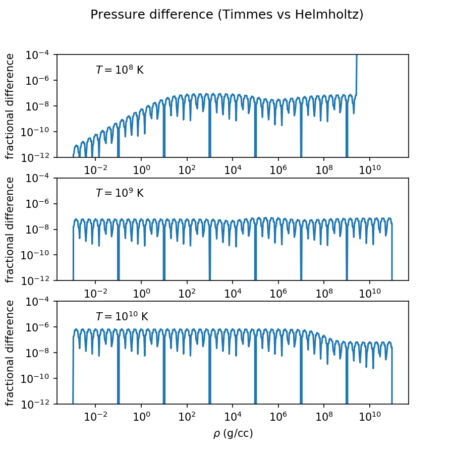
This also includes bindings to the Timmes EOS (but only in Rho-T basis).
If you use this code, please cite Timmes & Swesty (2000) and this software
.
You must have numpy and a fortran compiler installed. These bindings are constructed using f2py.
This is only tested on python3, though in principle one should be able to relatively easily adapt it to python2.
Python determines the module name using the path name, so you should change the root folder of this git repository to helmholtz. For example,
git clone git@github.com:jschwab/python-helmholtz.git helmholtz
The Makefile contains several relevant executable names and paths. The defaults are sensible, but you might need/want to edit them (for example, if your system appends “3” to python3 related executables).
FC=gfortran
F2PY=f2py
HELM_TABLE_DIR=$(shell pwd)
HELM_TABLE_NAME=helm_table.dat
Then in this directory, simply type
make module
and then add this directory to your python path
export PYTHONPATH=/path/to/module:$PYTHONPATH
This code has only cosmetic changes from the version of helmholtz provided on Frank Timmes website (last updated 2018-12-10).
- Set ionization variables irowmax and jstagemax to 1
- Set nrowmax to 1,000,000 (allowing large arrays)
- Set path to helm_table.dat at compile time
At least in theory, updates can be performed by simply untar-ing a new version of helmholtz and accepting all code changes except for these.
import numpy as np
import matplotlib.pyplot as plt

import helmholtz

d = np.logspace(-3, 11, 512)
ts = [1e8, 1e9, 1e10]

fig, axs = plt.subplots(3)

for ax, t in zip(axs, ts):

    f = helmholtz.eosfxt(dens=d, temp=t, abar=1.0, zbar=1.0)
    h = helmholtz.helmeos(dens=d, temp=t, abar=1.0, zbar=1.0)

    ax.plot(d, np.abs((h.ptot - f.ptot)/f.ptot))
    ax.set_xlabel(r'$\rho$ (g/cc)')
    ax.set_ylabel(r'fractional difference')
    ax.set_xscale('log')
    ax.set_yscale('log')
    ax.set_ylim(1e-12, 1e0)

    logT = int(np.log10(t))
    ax.text(1e-2, 3e-6, '$T = 10^{{{}}}$ K'.format(logT))

fig.suptitle('Pressure difference (Timmes vs Helmholtz)')
fig.set_size_inches(6,6)
fig.savefig('fig1.png', dpi=150)Josiah Schwab <jschwab at gmail dot com>
