Juan Fonseca
This work is based on data from OpenPrescribing.
Loading the libraries for this analysis
library(sf)Linking to GEOS 3.11.2, GDAL 3.8.2, PROJ 9.3.1; sf_use_s2() is TRUE
library(tidyverse)── Attaching core tidyverse packages ──────────────────────── tidyverse 2.0.0 ──
✔ dplyr 1.1.4 ✔ readr 2.1.5
✔ forcats 1.0.0 ✔ stringr 1.5.1
✔ ggplot2 3.5.1 ✔ tibble 3.2.1
✔ lubridate 1.9.3 ✔ tidyr 1.3.1
✔ purrr 1.0.2
── Conflicts ────────────────────────────────────────── tidyverse_conflicts() ──
✖ dplyr::filter() masks stats::filter()
✖ dplyr::lag() masks stats::lag()
ℹ Use the conflicted package (<http://conflicted.r-lib.org/>) to force all conflicts to become errors
library(tmap)Breaking News: tmap 3.x is retiring. Please test v4, e.g. with
remotes::install_github('r-tmap/tmap')
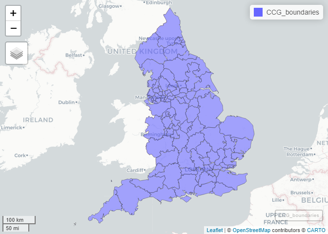
Practices are grouped in sub-ICB. The following code extracts the boundaries for all ICBs in the country
CCG_boundaries <- geojsonsf::geojson_sf("https://openprescribing.net/api/1.0/org_location/?org_type=ccg") Warning in readLines(con): incomplete final line found on
'https://openprescribing.net/api/1.0/org_location/?org_type=ccg'
mapview::mapview(CCG_boundaries)Approximate locations of all registered GP surgeries can also be
extracted. For example, let’s find the code for Leeds (ICB code: 15F )
CCG_boundaries |>
  st_drop_geometry() |>
  filter(str_detect(name,"LEEDS"))
name code ons_code org_type
1 NHS LEEDS 15F <NA> CCG
Creating a variable for the code and assigning the code for Leeds
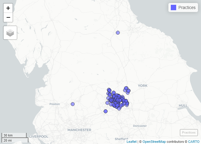
ICB_code <- "15F" Extracting the data for the practices which is a geoJSON file.
Practices <- geojsonsf::geojson_sf(paste0(
  "https://openprescribing.net/api/1.0/org_location/?q=",
  ICB_code
  )) |>
  st_transform(27700)
Warning in readLines(con): incomplete final line found on
'https://openprescribing.net/api/1.0/org_location/?q=15F'
Plotting the data
mapview::mapview(Practices)There are two relevant metrics which are readily available:
-
Short acting beta agonist inhalers
-
High dose inhaled corticosteroids
The metrics are produced for each month. Producing a moving average is possible but it will requires to build the database with the raw data, also prescriptions have been normalised in the processed dataset.
See: https://openprescribing.net/measure/saba/definition/
Taken from the web:
Why it matters: Why Asthma Still Kills reports that high use of short acting beta agonists (salbutamol and terbutaline) and poor adherence to inhaled corticosteroids in asthma suggests poor control - these patients should be reviewed regularly to ensure good control.
The NHS England National Medicines Optimisation Opportunities for 2023/24 identify improving patient outcomes from the use of inhalers as an area for improvement.
Description: Prescribing of short acting beta agonist (SABA) inhalers - salbutamol and terbutaline - compared with prescribing of inhaled corticosteroid inhalers and SABA inhalers
The following code reads the SABA data for the ICB_code we have
already defined
saba <- read_csv(paste0(
  "https://openprescribing.net/api/1.0/measure_by_practice/?format=csv&org=",
  ICB_code,
  "&parent_org_type=ccg&measure=saba")
  )
Rows: 6832 Columns: 9
── Column specification ────────────────────────────────────────────────────────
Delimiter: ","
chr (4): measure, org_type, org_id, org_name
dbl (4): numerator, denominator, calc_value, percentile
date (1): date
ℹ Use `spec()` to retrieve the full column specification for this data.
ℹ Specify the column types or set `show_col_types = FALSE` to quiet this message.
See: https://openprescribing.net/measure/icsdose/definition/
Taken from the web:
Why it matters: Latest BTS/SIGN guidance on the treatment of asthma recommends that patients should be maintained at the lowest possible dose of inhaled corticosteroid. Reduction in inhaled corticosteroid dose should be slow as patients deteriorate at different rates. Reductions should be considered every three months, decreasing the dose by approximately 25–50% each time. This measure uses table 12 of the BTS/SIGN guidance to define which inhalers are considered high-dose.
The latest guidance for treatment of COPD now recommends use of another treatment in preference to inhaled corticosteroids. There is some evidence that inhaled corticosteroids increases the risk of pneumonia. This risk appears to increase with dose.
Description: Prescribing of high dose inhaled corticosteroids compared with prescribing of all inhaled corticosteroids
The following code reads the ICS data for the ICB_code we have already
defined
icsdose <- read_csv("https://openprescribing.net/api/1.0/measure_by_practice/?format=csv&org=15F&parent_org_type=ccg&measure=icsdose")Rows: 6832 Columns: 9
── Column specification ────────────────────────────────────────────────────────
Delimiter: ","
chr (4): measure, org_type, org_id, org_name
dbl (4): numerator, denominator, calc_value, percentile
date (1): date
ℹ Use `spec()` to retrieve the full column specification for this data.
ℹ Specify the column types or set `show_col_types = FALSE` to quiet this message.
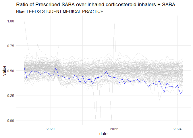
It is possible to extract the trends of both metrics. Below a graphical extract of one of the metrics for Leeds for a single GP practice.
head(saba)# A tibble: 6 × 9
measure org_type org_id org_name date numerator denominator calc_value
<chr> <chr> <chr> <chr> <date> <dbl> <dbl> <dbl>
1 saba practice B86071 WHITEHALL… 2019-03-01 413 734 0.563
2 saba practice B86041 VESPER RO… 2019-03-01 282 517 0.545
3 saba practice B86070 AIREBOROU… 2019-03-01 151 313 0.482
4 saba practice B86069 BURLEY PA… 2019-03-01 313 594 0.527
5 saba practice B86003 DR G LEES… 2019-03-01 611 1100 0.555
6 saba practice B86651 ONE MEDIC… 2019-03-01 0 0 NA
# ℹ 1 more variable: percentile <dbl>
saba |>
  ggplot(aes(x = date,
             y = calc_value,
             groups = org_id,
             col = mycol,
             alpha = myalpha))+
  geom_line(alpha = 0.4, col = "gray")+
  geom_line(data = saba[grep(pattern = "STUDENT",saba$org_name),],
            col = "blue",
            alpha = 0.8)+
  theme_minimal()+
  labs(title = "Ratio of Prescribed SABA over inhaled corticosteroid inhalers + SABA",
       y = "value",
       subtitle = "Blue: LEEDS STUDENT MEDICAL PRACTICE"
  )
Warning: Removed 1185 rows containing missing values or values outside the scale range
(`geom_line()`).
First let’s check the data quality for all practices and remove the NAs.
saba |>
  drop_na() |>
  summarise(n_reports = n(),
            .by = org_id) |>
  arrange(n_reports)
# A tibble: 101 × 2
org_id n_reports
<chr> <int>
1 Y00025 2
2 Y00683 3
3 B86095 4
4 B86047 7
5 B86682 8
6 B86077 9
7 B86633 13
8 B86031 15
9 B86023 30
10 B86074 36
# ℹ 91 more rows
We create a vector with the ids that have more than 10 records
ids_to_include <- saba |>
  drop_na() |>
  summarise(n_reports = n(),
            .by = org_id) |>
  arrange(n_reports) |>
  filter(n_reports>10) |>
pull(org_id)Extracting the start month from the dataset
start_month <- min(saba$date)Defining a function to calculate the month number of the record
diff_month <- function(start, end){
  length(seq(from=start, to=end, by='month')) - 1
}
Calculating the month difference
saba$month <- vapply(saba$date,\(x){
diff_month(start_month,x)},numeric(1))We are interested only in the built-up areas. For this purpose, we will use the spatial data obtained from Ordnance Survey (Download it manually and save it in the same folder of this project)
builtup_bounds <- st_read("OS Open Built Up Areas.gpkg",
                          layer = "os_open_built_up_areas")
Reading layer `os_open_built_up_areas' from data source
`C:\Users\ts18jpf\OneDrive - University of Leeds\03_PhD\00_Misc_projects\Eng-Presc-Data\OS Open Built Up Areas.gpkg'
using driver `GPKG'
Simple feature collection with 8585 features and 7 fields
Geometry type: MULTIPOLYGON
Dimension: XY
Bounding box: xmin: 65300 ymin: 10000 xmax: 655625 ymax: 1177650
Projected CRS: OSGB36 / British National Grid
clean_data <- saba |>
  semi_join(Practices[builtup_bounds,] |>
              filter(code %in% ids_to_include),
            by = c("org_id"="code"))
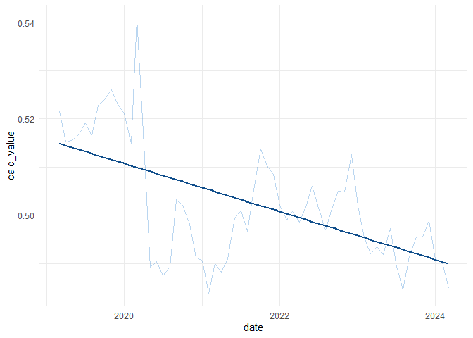
Calculating the overall trend in Leeds built-up areas
data_overall <- clean_data |>
  summarise(across(numerator:denominator,sum),
            .by = c(date, month)) |>
  mutate(calc_value = numerator/denominator)
data_overall |>
ggplot(aes(date,calc_value))+
geom_line(alpha = 0.3,
col = "dodgerblue3")+
geom_smooth(method = "lm",se = F,col = "dodgerblue4")+
theme_minimal()`geom_smooth()` using formula = 'y ~ x'
Fitting a simple linear model
lm(calc_value~month,data = data_overall) |>
  summary()
Call:
lm(formula = calc_value ~ month, data = data_overall)
Residuals:
Min 1Q Median 3Q Max
-0.0214383 -0.0042416 0.0009282 0.0062415 0.0309175
Coefficients:
Estimate Std. Error t value Pr(>|t|)
(Intercept) 5.149e-01 2.576e-03 199.875 < 2e-16 ***
month -4.158e-04 7.405e-05 -5.615 5.58e-07 ***
---
Signif. codes: 0 '***' 0.001 '**' 0.01 '*' 0.05 '.' 0.1 ' ' 1
Residual standard error: 0.01018 on 59 degrees of freedom
Multiple R-squared: 0.3483, Adjusted R-squared: 0.3372
F-statistic: 31.53 on 1 and 59 DF, p-value: 5.575e-07


