Build a Traffic Sign Recognition Project
The goals / steps of this project are the following:
- Load the data set (see below for links to the project data set)
- Explore, summarize and visualize the data set
- Design, train and test a model architecture
- Use the model to make predictions on new images
- Analyze the softmax probabilities of the new images
- Summarize the results with a written report
Here I will consider the rubric points individually and describe how I addressed each point in my implementation.
1. After importing the dataset files I mostly used the methods len() and shape() to calculate number of examples and the shape of the images. I also imported the names of the labels for the traffic signs using the CSV library.
- Number of training examples = len(X_train) = 34799
- Number of validation examples = len(X_valid) = 4410
- Number of testing examples = len(X_test) = 12630
- Image data shape = X_train[0].shape = (32, 32, 3)
- Number of classes = len(all_labels) = 43
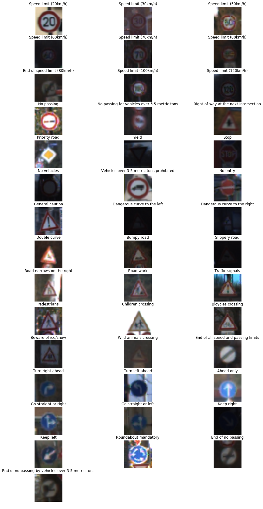
For the exploratory visualization of the data set. I first printed one image of each class with it correspondent label.
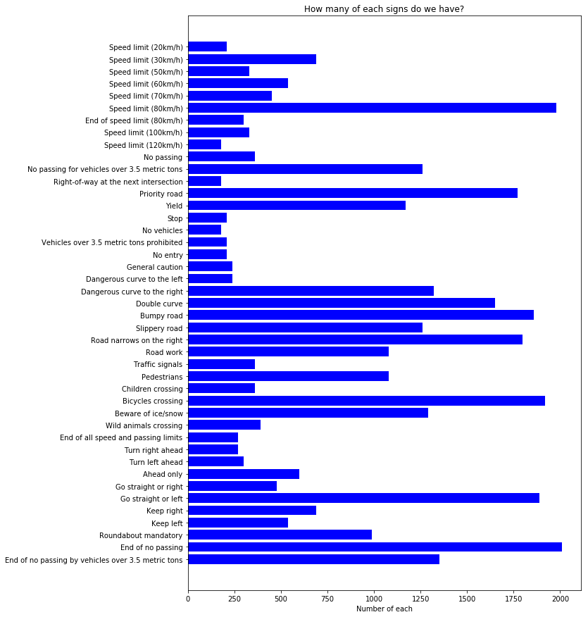
Then I printed a bar chart showing how many examples of each class were available on the training set.
As a first step, I decided to shuffle the examples using shuffle from the sklearn.utils library. X_train, y_train = shuffle(X_train, y_train)
As a last step, I normalized the image data because I was hoping to increase accuracy. I was surprised with the positive results.
I also tried augmenting the dataset, converting the examples to grayscale and transforming the image but non of this resulted on a better prediction. The normalization was the one that return better results and finally returned a model capable of classifying my own images correctly.
For my final model I used the LeNet example from Lesson 8. I change the Input from images with one channel to images with 3 channels and modified the number of labels from 10 to len(all_labels) which in this case was 43.
I tried using tf.nn.dropout but I wasn't able to achieve any substantial improvement on my training.
| Layer | Description |
|---|---|
| Input | 32x32x3 RGB image |
| Convolution 1 | 1x1 stride, VALID padding, output = 28x28x6 |
| RELU | |
| Max pooling | 2x2 stride, VALID padding, output = 14x14x6 |
| Convolution 2 | 1x1 stride, VALID padding, output = 10x10x16 |
| RELU | |
| Max pooling | 2x2 stride, VALID padding, output = 5x5x16 |
| Flatten | output = 400 |
| Fully connected | input = 400, output = 120 |
| RELU | |
| Fully connected | input = 120, output = 84 |
| RELU | |
| Fully connected | input = 84, output = 10 |
To train the model I used 20 epochs, a batch size of 128 and a learning rate of 0.001.
For my training optimizers I used softmax_cross_entropy_with_logits to get a tensor representing the mean loss value to which I applied tf.reduce_mean to compute the mean of elements across dimensions of the result. Finally I applied minimize to the AdamOptimizer of the previous result.
My final model Validation Accuracy was 0.958
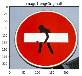
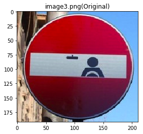
I choose seven German traffic signs found on the web and specially some that were altered on funny ways.
Here are 2 of the altered German traffic signs that I found on the web:
To make sure that
Here are the results of the prediction:
| Image | Prediction |
|---|---|
| No entry | No entry |
| Yield | Yield |
| No entry | No entry |
| No entry | No entry |
| Stop | Stop |
| Speed limit (70km/h) | Speed limit (30km/h) |
| Keep Right | Priority road |
The model was able to correctly predict 5 other 7 traffic signs, which gives an accuracy of 71%.
Based on the comparison with the accuracy of the testing sample (0.958) and the lower number of images for Speed limit 70 in contrast with other speed limits images I think the bad prediction of the max speed sign was due the small quantity of examples for this kind of images on the data sample. Adding variations of the images by inverting, rotating or augmenting the them might have increased the accuracy.
####3. Describe how certain the model is when predicting on each of the five new images by looking at the softmax probabilities for each prediction. Provide the top 5 softmax probabilities for each image along with the sign type of each probability. (OPTIONAL: as described in the "Stand Out Suggestions" part of the rubric, visualizations can also be provided such as bar charts)
The code for making predictions on my final model is located in the 11th cell of the Ipython notebook.
For my images 1, 2, 3 and 5 my model was 100% sure that the results were correct. For image number 3 the probability was 79.41% and still got it right. For images 6 and 7 the probability was 93.64% and 92.08% but it got them wrong. For image number 6 the second option was the correct one but for image number 7 the correct solution wasn't listed in the top 5 softmax.
image1.png: No entry: 100.00% Speed limit (120km/h): 0.00% Traffic signals: 0.00% Stop: 0.00% Children crossing: 0.00%
image2.png: Yield: 100.00% Priority road: 0.00% No passing for vehicles over 3.5 metric tons: 0.00% Speed limit (50km/h): 0.00% Speed limit (20km/h): 0.00%
image3.png: No entry: 79.41% Stop: 9.97% Traffic signals: 4.87% Children crossing: 4.53% No vehicles: 1.23%
image4.jpg: No entry: 100.00% Speed limit (20km/h): 0.00% Speed limit (30km/h): 0.00% Speed limit (50km/h): 0.00% Speed limit (60km/h): 0.00%
image5.png: Stop: 100.00% Bicycles crossing: 0.00% Road work: 0.00% Bumpy road: 0.00% Children crossing: 0.00%
image6.png: Speed limit (30km/h): 93.64% Yield: 6.25% Speed limit (50km/h): 0.11% Speed limit (20km/h): 0.00% Dangerous curve to the right: 0.00%
image7.png: Priority road: 92.08% Keep right: 7.54% Speed limit (30km/h): 0.21% Speed limit (20km/h): 0.18% Roundabout mandatory: 0.00%
The challenge here was to name the convolutional step correctly so you can reference it from the get_tensor_by_name() function.q
After that it was easy to show one or more steps on the network.
Here is my results at the end of the first and second convolution using my web images:
1 - I would reduce the number of epochs to prevent it from going up and down on the prediction accuracy.
2 - I think the bad prediction of the max speed sign was due the small quantity of examples for this kind of images on the data sample. Adding variations of the images by inverting, rotating or augmenting the them might have increased the accuracy.


