Towards robust neural ODEs using parametrized solvers.
Each Runge-Kutta (RK) solver with s stages and of the p-th order is defined by a table of coefficients (Butcher tableau). For s=p=2, s=p=3 and s=p=4 all coefficient in the table can be parametrized with no more than two variables [1].
Usually, during neural ODE training RK solver with fixed Butcher tableau is used, and only the right-hand side (RHS) function is trained. We propose to use the whole parametric family of RK solvers to improve robustness of neural ODEs.
- pytorch==1.7
- apex==0.1 (for training)
For CIFAR-10 and MNIST demo, please, check examples folder.
In the notebook examples/cifar10/Evaluate model.ipynb we show how to perform the forward pass through the Neural ODE using different types of Meta Solver regimes, namely
- Standalone
- Solver switching/smoothing
- Solver ensembling
- Model ensembling
In more details, usage of different regimes means
-
Standalone
- Use one solver during inference.
- This regime is applied in the training and testing stages.
-
Solver switching / smoothing
- For each batch one solver is chosen from a group of solvers with finite (in switching regime) or infinite (in smoothing regime) number of candidates.
- This regime is applied in the training stage
-
Solver ensembling
- Use several solvers durung inference.
- Outputs of ODE Block (obtained with different solvers) are averaged before propagating through the next layer.
- This regime is applied in the training and testing stages.
-
Model ensembling
- Use several solvers durung inference.
- Model probabilites obtained via propagation with different solvers are averaged to get the final result.
- This regime is applied in the training and testing stages.
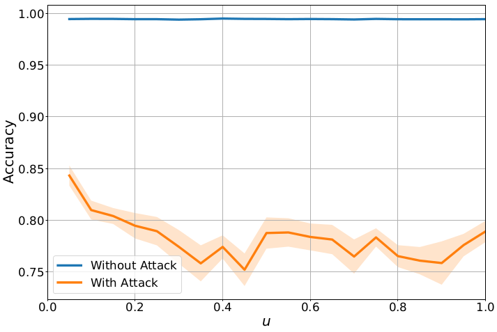
We have trained a neural ODE model several times, using different u values in parametrization of the 2-nd order Runge-Kutta solver. The image below depicts robust accuracies for the MNIST classification task. We use PGD attack (eps=0.3, lr=2/255 and iters=7). The mean values of robust accuracy (bold lines) and +- standard error mean (shaded region) computed across 9 random seeds are shown in this image.
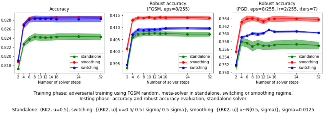
We compare results of neural ODE adversarial training on CIFAR-10 dataset with meta-solver in standalone, switching or smoothing regimes. We choose 8-steps RK2 solvers for this experiment.
- We perform training using FGSM random technique described in https://arxiv.org/abs/2001.03994 (with eps=8/255, alpha=10/255).
- We use cyclic learning rate schedule with one cycle (36 epochs, max_lr=0.1, base_lr=1e-7).
- We measure robust accuracy of resulting models after FGSM (eps=8/255) and PGD (eps=8/255, lr=2/255, iters=7) attacks.
- We use
premetanode10architecture fromsopa/src/models/odenet_cifar10/layers.pythat has the following formConv -> PreResNet block -> ODE block -> PreResNet block -> ODE block -> GeLU -> Average Pooling -> Fully Connected - We compute mean and standard error across 3 random seeds.

