Enhancing the Robustness via Adversarial Learning and Joint Spatial-Temporal Embeddings in Traffic Forecasting

This is the official Pytorch implementation for our CIKM 2023 paper: "TrendGCN: Enhancing the Robustness via Adversarial Learning and Joint Spatial-temporal Embeddings in Traffic Forecasting".

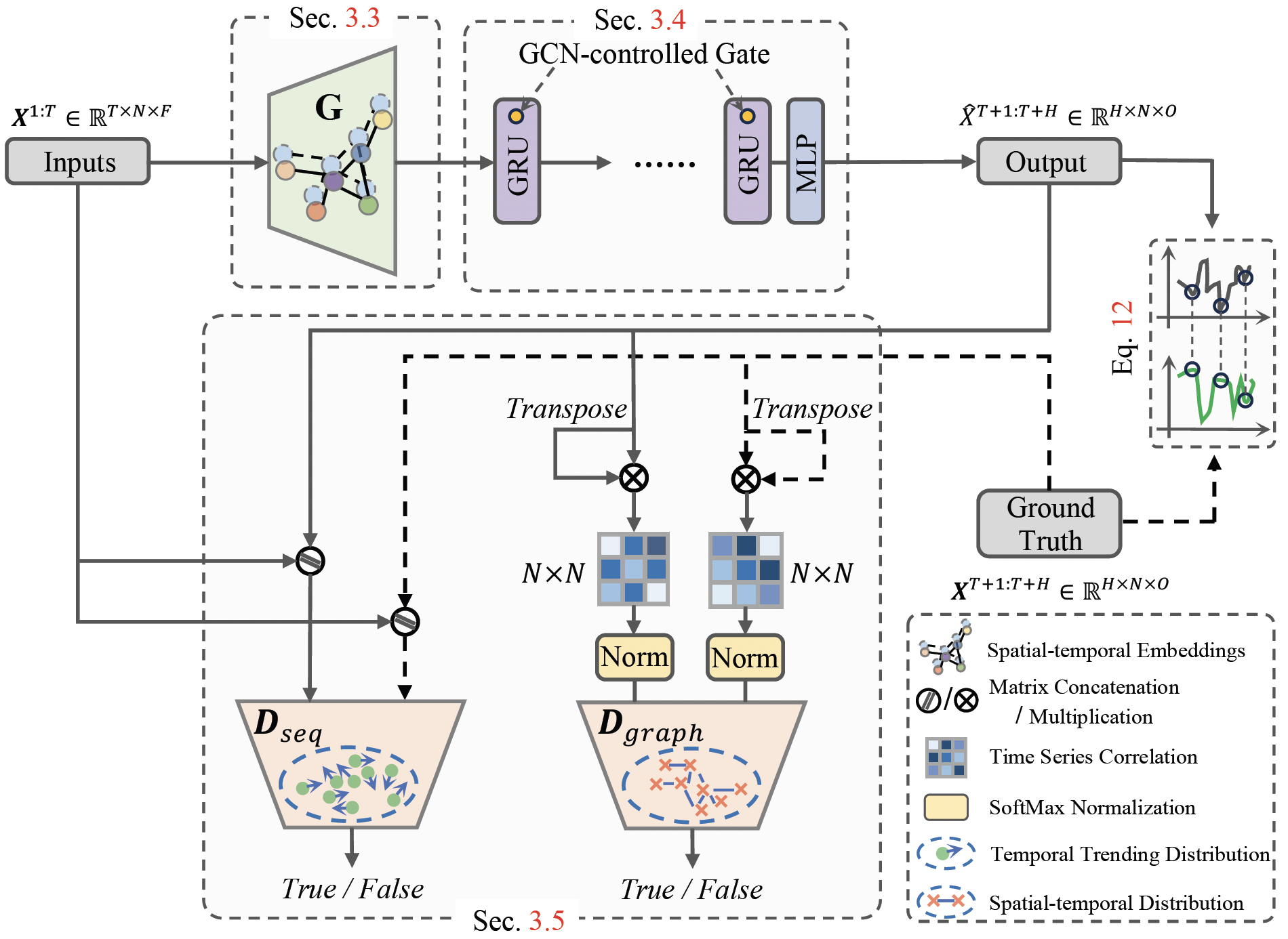
Figure 1. TrendGCN Model Architecture.

Overview

TrendGCN
├── config                   # the configuration of six datasets
    ├── METR-LA.conf
    ├── PEMS-Bay.conf
    ├── PEMS03.conf
    ├── PEMS04.conf
    ├── PEMS07.conf
    └── PEMS08.conf
├── dataset                  # place six dataset folders
    ├── METR-LA
    ├── PEMS-Bay
    ├── PEMS03
    ├── PEMS04
    ├── PEMS07
    └── PEMS08
├── model
    ├── discriminator.py     
    └── generator.py         
├── utils
    ├── adj_dis_matrix.py    # construct adjacent matrix 
    ├── metrics.py           # evaluation metrics
    ├── norm.py              # data normalization
    └── util.py              # useful tools
├── dataloader.py            # load dataset
├── LICENSE                  
├── main.py                  # run
├── README.md                # detailed illustration of model training and testing
├── requirements.yml         # environment dependencies
└── trainer.py               # training and testing procedure

Environment

Make sure you have Python>=3.8 and Pytorch>=1.8 installed on your machine.

Pytorch 1.8.1
Python 3.8.*

Install python dependencies by running:

conda env create -f requirements.yml
# After creating environment, activate it
conda activate trendgcn

Datasets Preparation

In our work, we evaluate proposed models on six real-world traffic benchmark dataset, including: PEMS03, PEMS04, PEMS07, PEMS08, PEMS-Bay, and METR-LA. Then, place them into dataset folder.

Train and Test

Step 1:

Modifying the following variables in main.py script.

#********************************************************#
Mode = 'Train'     # or Test (loading best_model.pth to evaluate on test dataset)
DATASET = 'PEMS04' # PEMS03 or PEMS04 or PEMS07 or PEMS08
#********************************************************#

Step 2:

Modifying corresponding configuration for used dataset at config/dataset_name.conf, e.g., config/PEMS04.conf.

[data]
num_nodes = 307
lag = 12
horizon = 12
val_ratio = 0.2
test_ratio = 0.2
tod = False
normalizer = std
column_wise = False
default_graph = True
...

Step 3:

python -u main.py --gpu_id=1 2>&1 | tee exps/PEMS04.log

Note that for descriptions of more arguments, please run python main.py -h. After training, the model will be evalutated on test dataset automatically. The results for 1 ~ 12 horizon prediction will be shown in terminal or can be found in the end of exps/PEMS04.log.

Horizon 01, MAE: 17.16, RMSE: 27.69, MAPE: 11.2595%
Horizon 02, MAE: 17.57, RMSE: 28.50, MAPE: 11.4979%
Horizon 03, MAE: 17.98, RMSE: 29.21, MAPE: 11.7343%
Horizon 04, MAE: 18.29, RMSE: 29.76, MAPE: 11.9162%
Horizon 05, MAE: 18.54, RMSE: 30.23, MAPE: 12.0755%
Horizon 06, MAE: 18.80, RMSE: 30.68, MAPE: 12.2436%
Horizon 07, MAE: 19.04, RMSE: 31.09, MAPE: 12.4009%
Horizon 08, MAE: 19.24, RMSE: 31.43, MAPE: 12.5158%
Horizon 09, MAE: 19.43, RMSE: 31.76, MAPE: 12.6333%
Horizon 10, MAE: 19.62, RMSE: 32.05, MAPE: 12.7421%
Horizon 11, MAE: 19.82, RMSE: 32.37, MAPE: 12.8842%
Horizon 12, MAE: 20.20, RMSE: 32.88, MAPE: 13.1226%
Average Horizon, MAE: 18.81, RMSE: 30.68, MAPE: 12.2522%

More prediction results are stored in exps/META-LA.log, exps/PeMS-BAY.log, exps/PEMS03.log, exps/PEMS07.log, and exps/PEMS08.log.

Experimental Results

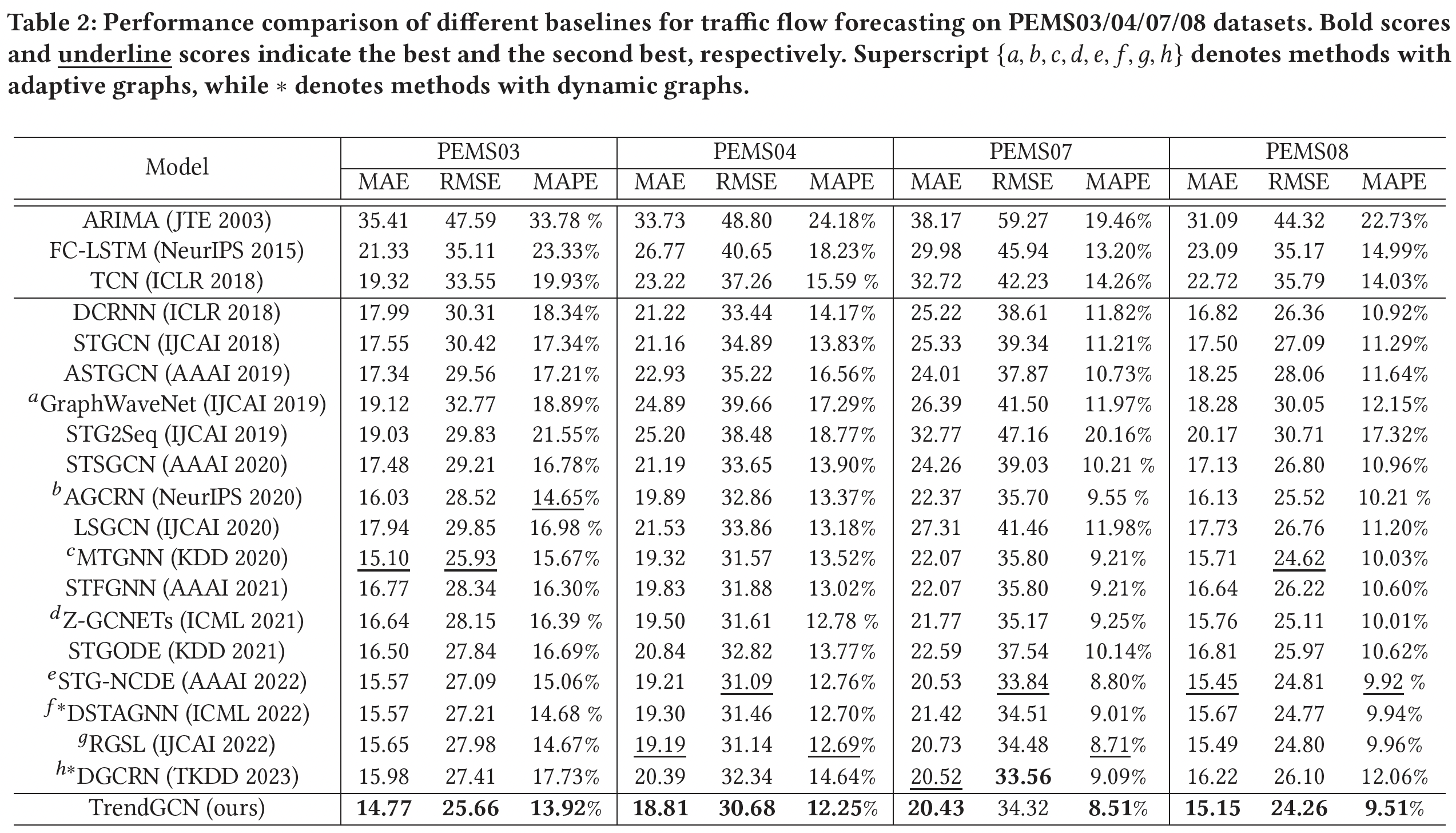
The prediction average horizon results of TrendGCN on six datasets are as follows:

Visualization

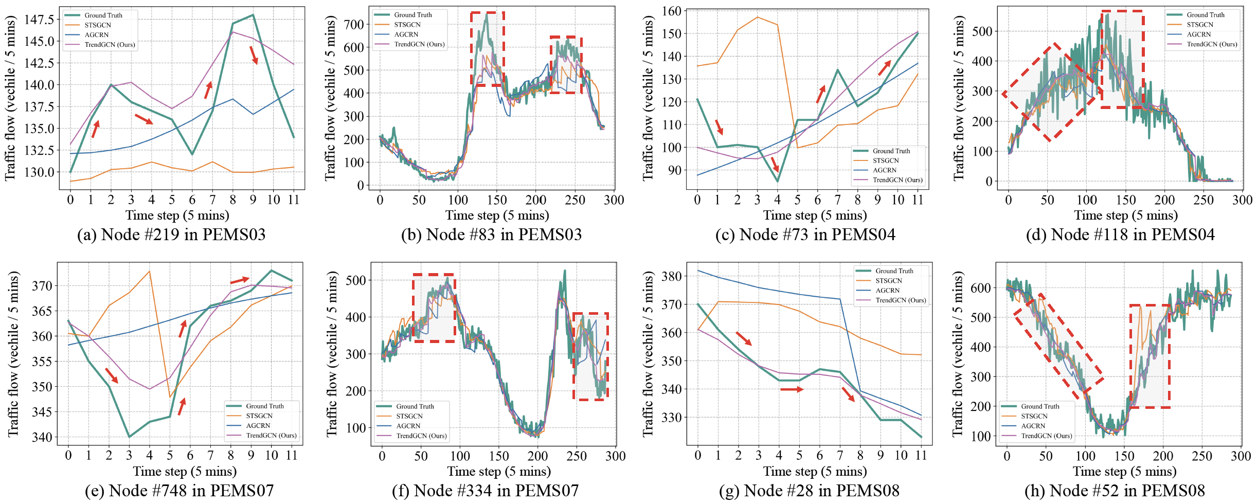
Figure 2. Comparison of short (12 steps)-(a)(c)(e)(g) and long (288 steps)-(b)(d)(f)(h) term prediction curves between STSGCN, AGCRN, and our TrendGCN on a snapshot of the test data of four datasets. Note that, the predicted time series for the whole day period (288 steps) is simply obtained by concatenating all the short-term predictions (12 steps) along the time axis (and remove overlaps), which is a common practice widely used in existing literatures, so that a better visualization of the prediction quality during different time of the day can be presented.

Figure 3. Visualization of 2D projection of UMAP on spatial embeddings (Upper) and the heatmap of learned graphs (Lower) at t = {2, 4, 6, 8, 10, 12} time steps.

Citation

If you use the data or code in this repo, please cite the repo.

@article{jiang2022dynamic,
  title={Enhancing the Robustness via Adversarial Learning and Joint Spatial-Temporal Embeddings in Traffic Forecasting},
  author={Jiang, Juyong and Wu, Binqing and Chen, Ling and Zhang, Kai and Kim, Sunghun},
  journal={arXiv preprint arXiv:2208.03063},
  year={2022}
}

juyongjiang/TrendGCN