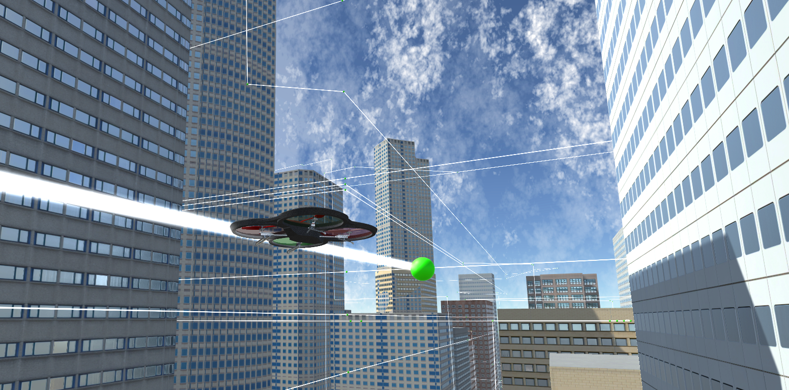
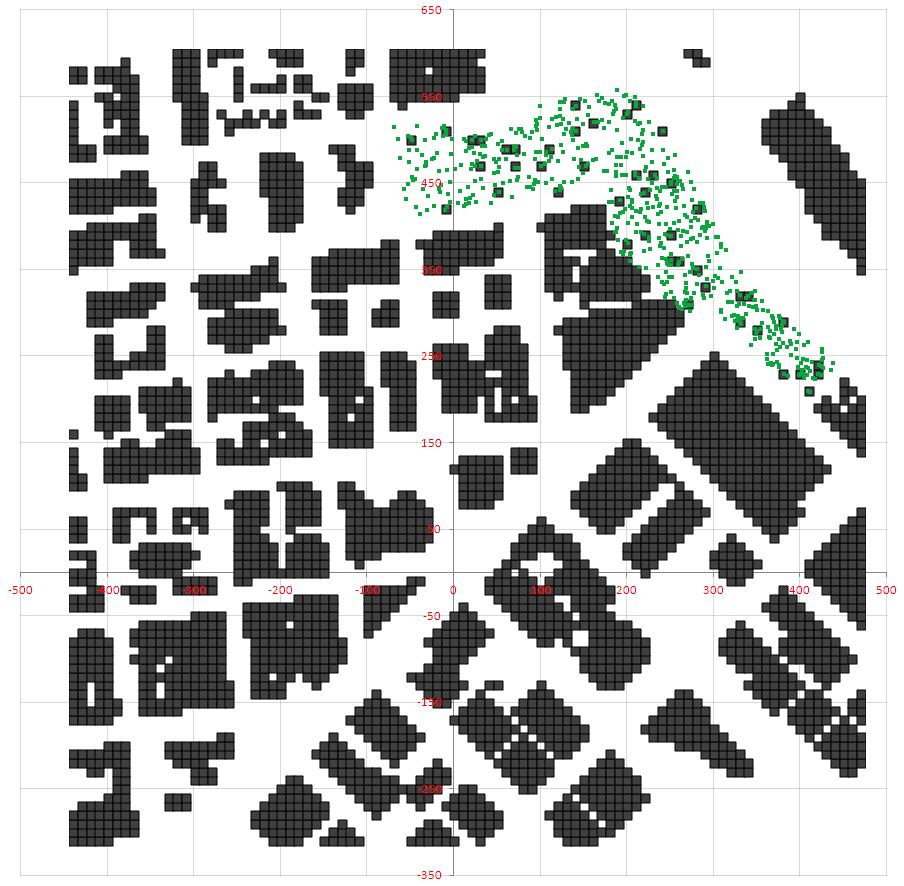
The goal of the project is to plan a path through an urban environment. The report following consists of 6 sections: starter code, initial implementation, executing test flights, additional functionality, potential optimizations, and references. See also the motion_planning.py script for reference.
The initial version of the motion_planning.py script is compared side-by-side with the backyard_flyer_solution.py script to briefly describe how each of the implemented modifications is functioning. See Figure 1 below.
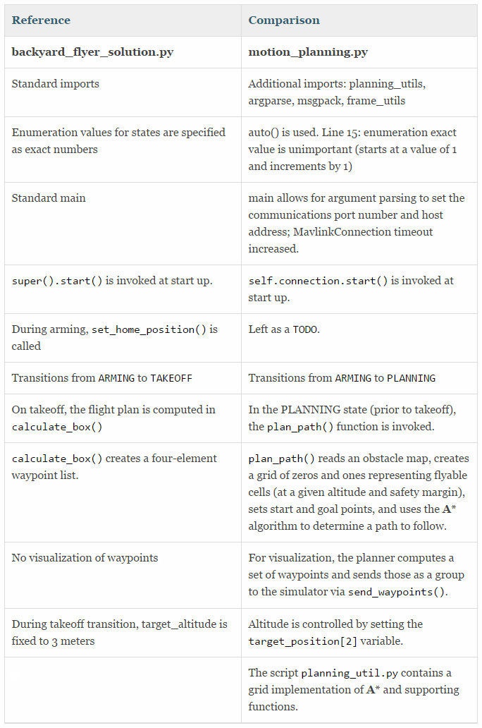
Figure 1: Comparison of starter code to backyard_flyer_solution.py
Set global home by reading the first line of the csv file, extracting lat0 and lon0 as floating point values and using the self.set_home_position() method. [at line 396 in motion_planning.py]
Retrieve current position in geodetic coordinates from self._latitude, self._longitude and self._altitude [at line 400 in motion_planning.py].
Set the start point as current location [at line 239 in motion_planning.py]
Set the goal point as any location on the grid [at 244 in motion_planning.py See also the options section starting at line 40].
Diagonal motions added to A* [at line 103 in planning_utils.py]. Additional features discussed below.
Cull waypoints from the grid paths using a 2D colinearity test [starting at line 244 in planning_utils.py]. Grid paths are pruned of excessive points by successively removing the middle point of three if they all fall on the same current line and share the same altitude. When a change in angle is detected, the middle point is retained. The variable self.cull enables pruning. (Graph paths are not pruned.)
Set the self.goal variable to a geodetic coordinate within the city. [See the options section starting at line 40 in motion_planning.py]
If the self.goal variable is set to None, then the program follows an itinerary of 222 coordinates listed in the file itinerary.csv. See Figure 2. The flying vehicle visits locations to "make deliveries and pickups". A further option (self.randomize_itin) allows for randomization of the itinerary. For test purposes, an option (self.visit_first) will ensure an initial visit to the specified index destination (even if randomization is in effect). Note: For itinerary travel, if n items are listed in the file, then n number of stops will be performed.
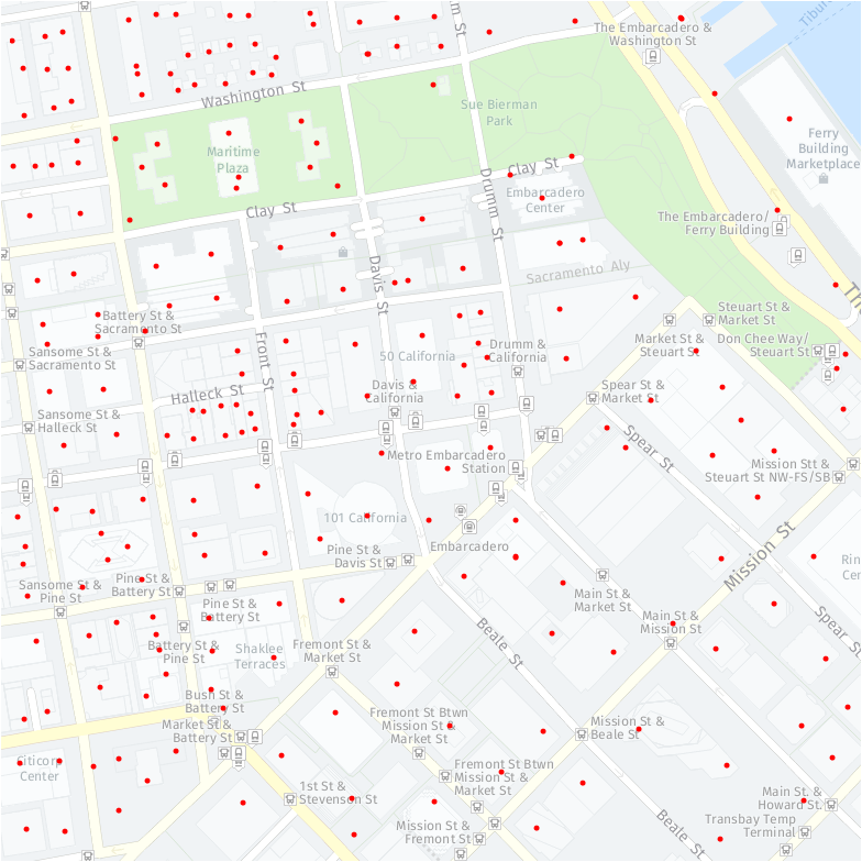
Figure 2: The itinerary contains 222 stops within the city (indicated as red dots).
Collider issue: From the rubric: "At the moment there is some mismatch between the colliders map and actual buildings in the scene." See Figure 3. If a random position is specified, the closest safe landing position is selected from the itinerary. This can be overridden (self.snap) at risk of unsafe landings (such as half-way onto a building roof or ledge).
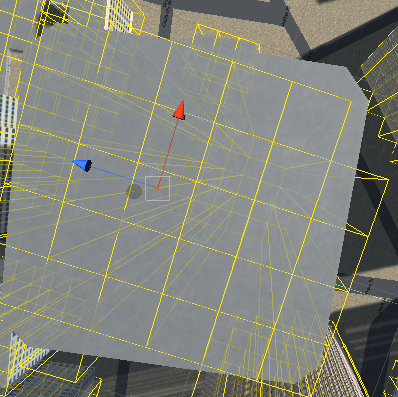
Figure 3: Misalignment of collider map (shown in yellow)
Grid improvements
Finding a pathway from some starting positions such as building courtyards proved to be challenging. Two code modifications overcome this: 1) the Grid class operates as a 2.5D model of the terrain, and 2) the A* algorithm accounts for altitude changes as an additional cost. Thus, buildings are considered as obstacles to go over or around, not dead ends. There are some building courtyards where the colliders are not aligned to the building properly, so a larger safety distance may be required for proper departure. However, an increase in safety distance may also complicate targeting of courtyards. A separate grid without safety distance is constructed to determine landing heights.
CLIMB_COST controls the cost of altitude changes. Presently set to a value of 100.0, this is tuned to fly "around" buildings most of the time and to fly "over" only when necessary. A question remains: What is the energy cost savings to fly around versus over?
Alternative heuristics functions are available for exploration: euclidean, manhattan, chebyshev, and octile. The octile function is tuned for a lower error estimation, however the Manhattan function is fast and sufficient.
Deadband radius is set to 5 meters for smoother waypoint acquisition.
Heading is calculated between waypoints as atan2(dy,dx) where dy is the difference in heading east and dx in heading north.
When operating with the graph-mode disabled (discussed next) the modified grid A* creates interesting pathways through the city. If the target altitude is higher than the departing altitude, the algorithm will seek increasingly direct routes as it climbs intermediate waypoints along the path.
Graph overlay option
- sampled geodetic coordinates at each major road intersection (see Figure 4)
- identified connecting bidirectional edges
- created supporting scripts to determine closest access points to the graph
- modified a copy of A* to operate with graph
- created compound path maker (grid/graph/grid)
- the
self.fly_lowvariable enables an altitude drop (to a minimum of 11 meters) while flying along graph edges. If disabled, the vehicle will fly at the altitude of the last departure location. - if the start and goal location share the same nearest graph node, then a direct route is planned without the graph.
- if the start and goal location are within a distance specified by
GRAPH_THRESHOLD, then a direct route is planned without the graph. This distance is set at 222 meters (a little more than the diagonal distance of one city block).
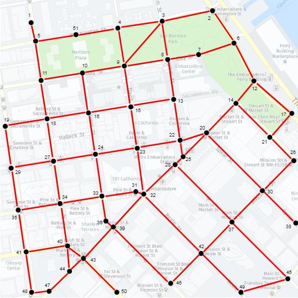
Figure 4: Graph visualization using draw.io. Nodes (black) are major intersections. Edges (red) mostly align with roads.
Advantages of the graph
- less time searching the grid (e.g. a few hundred cycles vs hundreds of thousands)
- higher performance
- road corridors are open and wide (less course corrections)
- avoids back alleys and congested building spaces
- each node "services" an area of the city
Disadvantages of the graph
- sometimes the closest node found can cause overshoot backtracking
- taller buildings cause some deeper search (but less than grid-only)
- lower cost routes are possible at higher altitudes
Converted obstacle grid into a class for re-usability. Also modified to store building height data rather than simple binary for a given altitude.
Tested some of the more challenging building courtyards - entrapments - pinchpoint alley-ways where colliders resolution may indicate an embedded area. See Figure 5.
Figure 5: Collider visualization in Excel with local coordinates at ground level.
Edge bisection: If a target lies between two nodes, an edge which spans the nodes could be split dynamically.
Acute angle edit: If a path includes an angle less than 45 degrees, a shorter path may be computed to optimize.
Edge cross-connection: When operating at higher altitudes, line-of-sight paths can reduce cost. This could be implemented as a multi-dimensional graph, where shortest paths may be identified at higher altitudes.
Plan memoization: Save and reuse previous paths; void with new obstacles.
Thoughts on Pathfinding
Amit Patel
http://theory.stanford.edu/~amitp/GameProgramming/Heuristics.html
Interactive pathfinding visualization
Xueqiao (Joe) Xu
https://qiao.github.io/PathFinding.js/visual/
Graph Search Algorithms
Steve Mussmann and Abi See
https://cs.stanford.edu/people/abisee/gs.pdf
Chebyshev distance
https://en.wikipedia.org/wiki/Chebyshev_distance
Alpha max plus beta min algorithm https://en.wikipedia.org/wiki/Alpha_max_plus_beta_min_algorithm
Development of a Three Dimensional Path Planner for Aerial Robotic Workers
Anastasios Zompas
http://essay.utwente.nl/71490/1/ZOMPAS_MA_EWI.pdf
Downtown San Francisco map
© 2018 HERE
https://wego.here.com/?map=37.79285,-122.39558,17,normal
