Aggressive Training of Inference Network

This is PyTorch implementation of the paper:

Lagging Inference Networks and Posterior Collapse in Variational Autoencoders
Junxian He, Daniel Spokoyny, Graham Neubig, Taylor Berg-Kirkpatrick
ICLR 2019

The code seperates optimization of encoder and decoder in VAE, and performs more steps of encoder update in each iteration. This new training procedure mitigates the issue of posterior collapse in VAE and leads to a better VAE model, without changing model components and training objective.

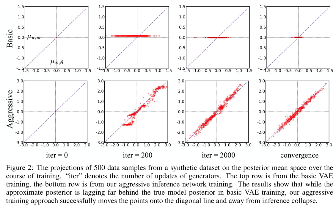
This repo is able to reproduce quantitative experimental results and qualitative visualizations of posterior mean space presented in the paper.

Please contact junxianh@cs.cmu.edu if you have any questions.

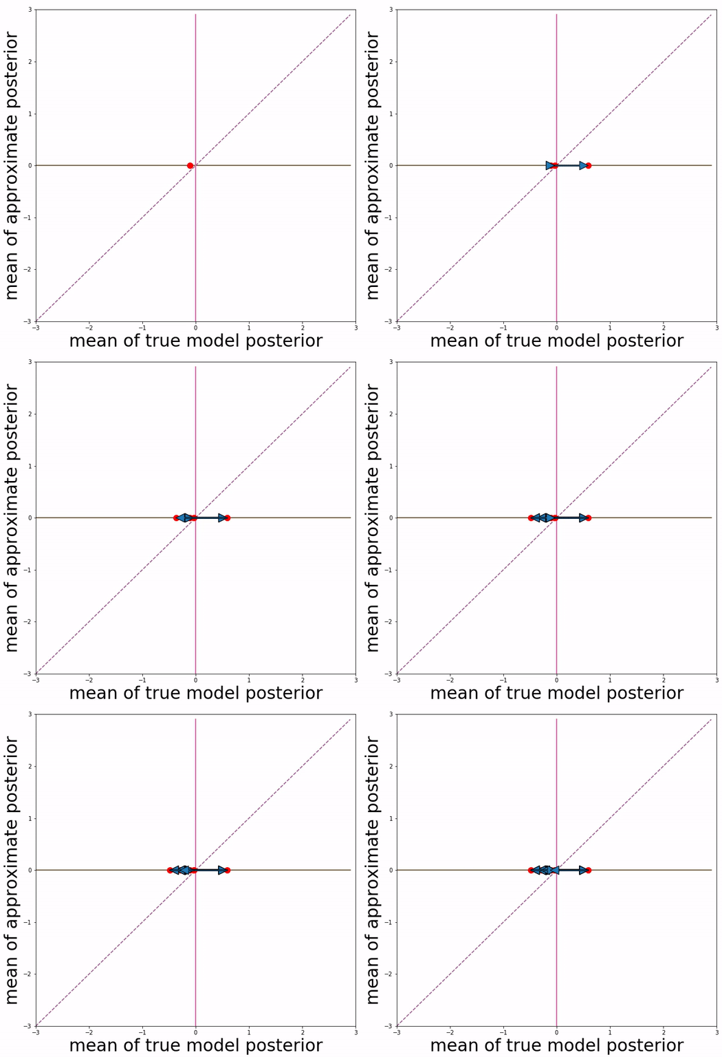
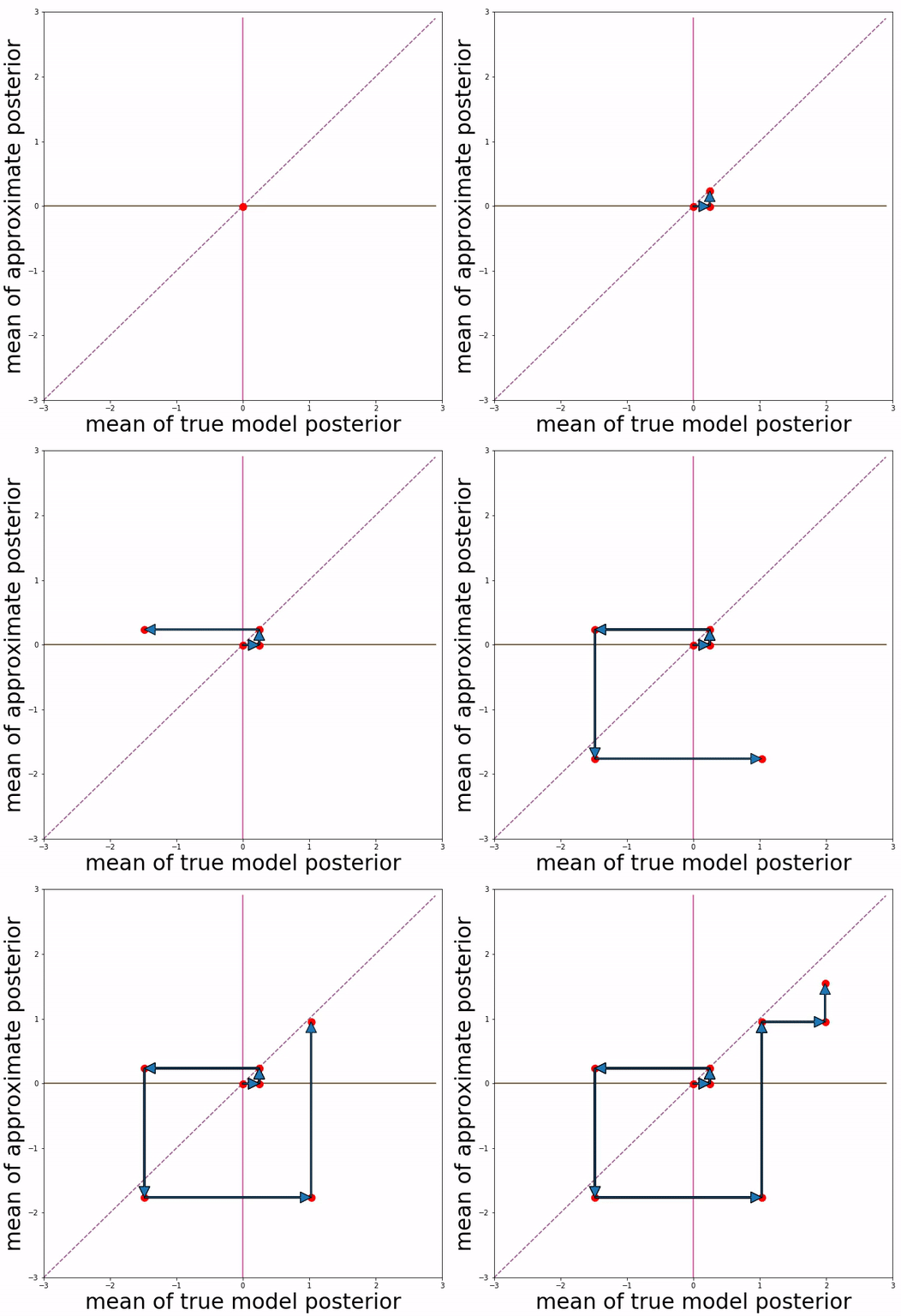
(a) basic VAE training (b) Aggressive VAE training

Posterior Mean Space

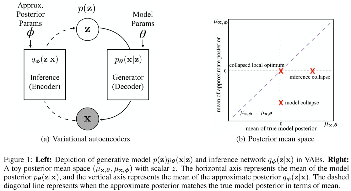
Our approach is inspired by the definition of "posterior mean space", which helps observe the posterior status over course of training and analyze VAE training behavior from the perspective of training dynamics. In the paper we experimented with a toy dataset and a scalar latent variable, so that posterior mean space is on a 2-d plane.

Requirements

Python >= 3.6
PyTorch >= 0.4

Data

Datasets used in this paper can be downloaded with:

python prepare_data.py

By default it downloads all four datasets used in the paper, downloaded data is located in ./datasets/. A --dataset option can be provided to specify the dataset name to be downloaded:

python prepare_data.py --dataset yahoo

The argument should be synthetic, yahoo, yelp, or omniglot.

Usage

Example script to train VAE on text data (training uses GPU when available):

python text.py --dataset yahoo --aggressive 1 --warm_up 10 --kl_start 0.1

image data:

python image.py --dataset omniglot --aggressive 1 --warm_up 10 --kl_start 0.1

Logs would be printed on standard output and also saved into folder logs.

Here:

--dataset specifies the dataset name, currently it supports synthetic, yahoo, yelp for text.py and omniglot for image.py
--aggressive controls whether applies aggressive training or not
--kl_start represents starting KL weight (set to 1.0 to disable KL annealing)
--warm_up represents number of annealing epochs (KL weight increases from kl_start to 1.0 linearly in the first warm_up epochs)

To run the code on your own text/image dataset, you need to create a new configuration file in ./config/ folder to specifiy network hyperparameters and datapath. If the new config file is ./config/config_abc.py, then --dataset needs to be set as abc accordingly.

Visualization of Posterior Mean Space

We project 500 data samples onto posterior mean space and observe the change over course of training.

To reproduce this visualization figure, first train the model on the toy dataset to save statistics required for visualization (training uses GPU when available):

python toy.py --aggressive 1 --plot_mode multiple

Here --plot_mode can be specified as single to reproduce the single-point trajectory figure (Figure 3 in the paper). This command trains a VAE model with aggressive training on synthetic data, and the required statistics is saved in folder plot_data (folder would be created automatically if non-existing).

Then run the plotting script:

python plot_scripts/plot_multiple.py --aggressive 1 --iter 2000

Here --aggressive specifies the aggressive training mode (should be the same as training), --iter specifies for which iteration the figure is plotted, we save the plotting data every 200 iterations by default at training time. The generated figures would be saved in folder plot_figure as pdf files (folder would be created automatically if non-existing).

Similarly, run plot_single.py is able to generate the single-point trajectory figure.

Text Generation

Text generation is supported through sampling from either the prior or posterior (i.e. reconstruction).

Generation from prior (by default it generates 100 samples):

python text.py --dataset [dataset] --decode_from [pretrained model path]

Reconstruction:

python text.py --dataset [dataset] --decode_from [pretrained model path] --decode_input [a text file for reconstruction]

--decode_input file has one raw sentence per line, which is the same format as training data.

Optional --decoding_strategy argument can be used to specifiy decoding strategy as {greedy, beam, sample}. By default greedy decoding is performed. Generated sentences are saved in folder samples.

Mutual Information and KL Curve

To plot the KL and mutual information curves over course of training (Figure 5 in the paper), first run:

python text.py --dataset yelp --aggressive 1 --warm_up 10 --kl_start 1.0

Then please refer to plot_scripts/plot_log.ipynb as an example to read the log file and generate plots.

Reference

@inproceedings{he2018lagging,
title={Lagging Inference Networks and Posterior Collapse in Variational Autoencoders},
author={Junxian He and Daniel Spokoyny and Graham Neubig and Taylor Berg-Kirkpatrick},
booktitle={Proceedings of ICLR},
year={2019}
}

jxhe/vae-lagging-encoder