jyanglab/Workflow-for-Genome-wide-Mediation-Analysis

bio-protocol

Overview of mediation analysis Workflow

Installation

• Running environment:

  • The workflow was constructed based on the Linux system running the R v4.1.1.

• Required software and versions:

  • Rstudio

install.packages(c("data.table", "glmnet", "MASS", "rrBLUP", "parallel", 
                   "doParallel", "CompQuadForm", "circlize", "dplyr", "RcolorBrewer"))

Input Data

Required input data:

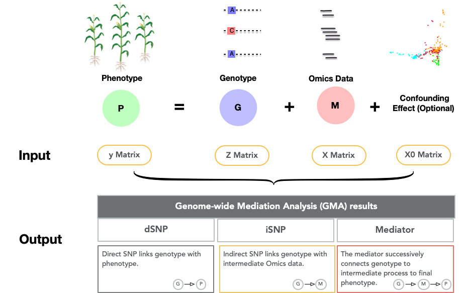
• y matrix (input/y_matrix.txt):
  • A n x 1 matrix of phenotype values; n is the number of individuals.

library("data.table")
y <- fread("input/y_matrix.txt", header=T,data.table=FALSE)
y = as.matrix(y)
dim(y) #271   1
head(y)

• Z matrix (input/Z_matrix.txt):
  • The n x m genotype matrix of data; m is the number of bi-allelic SNP markers, coded as -1, 0, 1.

Z <- fread("input/Z_matrix.txt", header=T,data.table=FALSE)
Z = as.matrix(Z)
dim(Z) #271 5000
Z[1:10, 1:10]

• X matrix (input/X_matrix.txt):
  • The n x k intermediate Omics matrix; k is the number of Omics traits. In the example, gene expression data (i.e., RNA-seq read counts of k genes) was used as the intermediate traits .

X <- fread("input/X_matrix.txt", header=T,data.table=FALSE)
X = as.matrix(X)
dim(X) #271 1200
X[1:10, 1:10]

Optional input data:

• X0 matrix (input/X0_matrix.txt):
  • A matrix of confounding effects. In the example, three principal components calculated from the Z matrix were used to control population structure.

X0 <- fread("input/X0_matrix.txt", header=T,data.table=FALSE)
X0 = as.matrix(X0)
dim(X0) #271   3
head(X0)
# X0 = prcomp(Z)$x[,1:3] # use this line of code to calculate principal components if no X0_matrix.txt file provided

---

Major steps

Step 1: Calculate confounding effect (or the X0 matrix)

Several principal components can be used as the fixed effects to control population structure as the confounding effects if using a structured population.

source('lib/utils.R')
        
Z <- fread("input/Z_matrix.txt", header=T, data.table=FALSE)
Z = as.matrix(Z)
X0 <- getpca(Z, p=3) # here the first p=3 PCs were extracted.

Step 2: Conduct GMA using different methods

#library(GMA)
library(glmnet)
library(MASS)
library(rrBLUP)
library(parallel)
library(doParallel)
library(CompQuadForm)
source('lib/highmed2019.r')
source('lib/fromSKAT.R')
source('lib/MedWrapper.R')
source('lib/reporters.R')

subX = X[, 1:100]
# run the fixed effect model that assign equal penalty on the two data types.
run_GMA(y, X0, subX, Z, ncores=10, model="MedFix_eq", output_folder="output/")

# run the fixed effect model that minimizes BIC
run_GMA(y, X0, subX, Z, ncores=10, model="MedFix_fixed", output_folder="output/")

# run the random effect model using linear kernel, and extract the model that minimizes BIC
run_GMA(y, X0, subX, Z, ncores=10, model="MedMix_linear", output_folder="output/")

# run the random effect model using shrink_EJ kernel, and extract the model that minimizes BIC
run_GMA(y, X0, subX, Z, ncores=10, model="MedMix_shrink", output_folder="output/")

Step 3: Visualize the results

library(circlize)
library(dplyr)
library("RColorBrewer")

gwas <- qGWAS(y, Z, plot=FALSE)
fwrite(gwas, "output/gwas_results.csv", sep=",", row.names = FALSE, quote=FALSE)


source("lib/circosplot.R")
circos_med(gwas_res="output/gwas_results.csv",
           med_res="output/mediators_fixed_bic_trait_V1.csv", 
           dsnp_res="output/dsnps_fixed_bic_trait_V1.csv", 
           isnp_res="output/isnps_fixed_bic_trait_V1.csv",
           chrlen="input/Chromosome_v4.txt", 
           gene_position= "input/gene_pos.csv",
           out_tiff = "graphs/circos.tiff")

Expected results

The outputs of the example data:

dSNP:

Direct SNPs identified using MedFix_eq and MedFix_fixed methods for trait V1. Note that only MedFix methods will report direct SNP.

• output/dSNP_MedFix_eq_trait_V1.csv
• output/dSNP_MedFix_fixed_trait_V1.csv

The dSNP output files contain the following columns:

• snp: direct SNP;
• pval: p-value of effect from exposure to outcome;
• coef: SNP effect from exposure to outcome.

iSNP:

Indirect SNPs identified. Again, only MedFix methods will report direct SNPs.

• output/iSNP_MedFix_eq_trait_V1.csv
• output/iSNP_MedFix_eq_trait_V1.csv

The iSNP output files contain the following columns:

• medi: mediator gene under control by the iSNP;
• snps_for_medi: indirect SNPs for the corresponding mediator;
• coef: effect from exposure to mediator.

Mediator:

The non-adjusted mediators detected by different methods of MedFix_BIC, MedFix_0.5, MedMixed_Linear, and MedMixed_Shrink for trait V1.

• output/mediator_MedFix_eq_trait_V1.csv
• output/mediator_MedFix_eq_trait_V1.csv
• output/mediator_MedMix_linear_trait_V1.csv
• output/mediator_MedFix_eq_trait_V1.csv:

The mediator output files contain the following columns:

• id: mediator gene id;
• e2m: p-value of effect from exposure to mediator;
• m2y: p-value of effect from mediator to outcome;
• e2m2y: maximum value between e2m and m2y;
• padj: adjusted p-value;
• coef: product of effect from exposure to mediator and effect from mediator to outcome.

Visualization of GMA results:

• In the circos plots, the outermost circular track represents the ten chromosomes;
• The next inner track shows the GWAS results, with two circular blue dashed lines indicating -log(p-value) of 5 and 10 and the red lines denoting the position of direct SNPs;
• The next inner track shows the relative positions of identified mediator genes with different genes represented by different colors; the lines in the innermost circle connects mediators with their corresponding indirect SNPs.

Citations

• Zhang, Qi. "High-dimensional mediation analysis with applications to causal gene identification." Statistics in Biosciences (2021): 1-20.
• Yang, Zhikai, Gen Xu, Qi Zhang, Toshihiro Obata, and Jinliang Yang. "Genome-wide mediation analysis: an empirical study to connect phenotype with genotype via intermediate transcriptomic data in maize." Genetics 221, no. 2 (2022): iyac057.

License

It is a free and open source software, licensed under GPLv3.