k-niss/bowtie

Construction of weighted topological overlap (wTO) matrices based on networks

Bowtie

This is an R package containing functions to construct and visualize weighted topological overlap (wTO) matrices based on weighted networks (tutorial part A). Functions for finding, extracting and highlighting protein complexes and bow-tie motif interaction fans are included as well (tutorial part B).

Table of Contents

Getting Started

Prerequisites

Tutorials

Authors

Affiliation

Publication

Acknowledgments

Getting Started

Make sure you have devtools installed and loaded:

install("devtools")
library("devtools")

Then install the bowtie package directly from github

install_github("k-niss/bowtie")
library("bowtie")

You may have to install the github repertoire using R in the terminal instead of in Rstudio. After that you can just restart Rstudio and load the library in the standard way using library(bowtie).

Prerequisites

Remember to install and then load the following packages before using the bowtie functions.

library("igraph")       # Graph package
library("reshape2")     # Matrix manipulation
library("pbapply")      # Apply functions with multiprocessing and progress bar
library("parallel")     # For multiprocessing
library("RColorBrewer") # Nice colors

Tutorials

In part A, we present how to calculate a wTO matrix based on an igraph object and followlingly how to visualize it. We use a toy network to reduce computation time of the tutorial. In part B, we illustrate how to extract protein complexes and knot proteins from a network adjacency matrix of direct interaction scores and how to visualize the results.

Tutorial part A: Creating and visualizing a wTO matrix

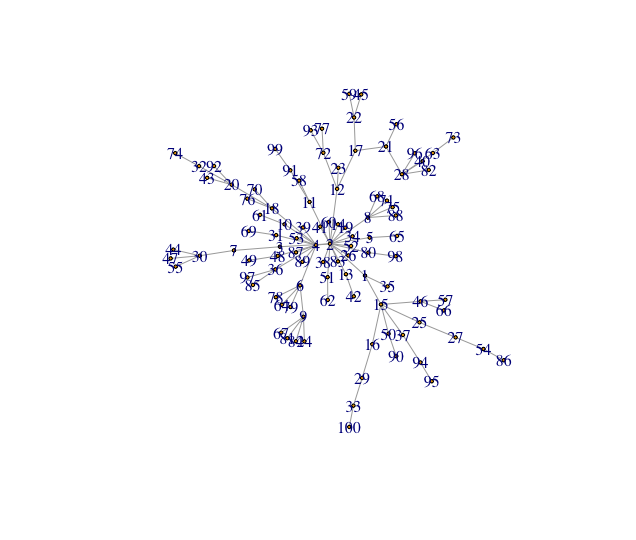
Create a toy network using the igraph function sample_pa() and visualize it:

random_graph           = sample_pa(n=100, power = 1.2, directed=F)
E(random_graph)$weight = runif(n=length(E(random_graph)))
plot(random_graph, vertex.size=2, layout=igraph::layout.gem(random_graph))

The algorithm will create a graph resembling the one above.

Calculate pariwise weighted topological overlap (wTO) for all node pairs:

wTO_list = wTO.network(node_vector=as.vector(V(random_graph)), igraph_object=random_graph, thread_numb=2)

Convert the list format into a symmetric wTO matrix:

wTO_matrix = from.list.to.df(wTO_list)

Order the columns and rows of the matrix, to make patterns stand out:

hclust_object = hclust(as.dist(1-wTO_matrix), method='average')
node_order    = hclust_object$labels[hclust_object$order]

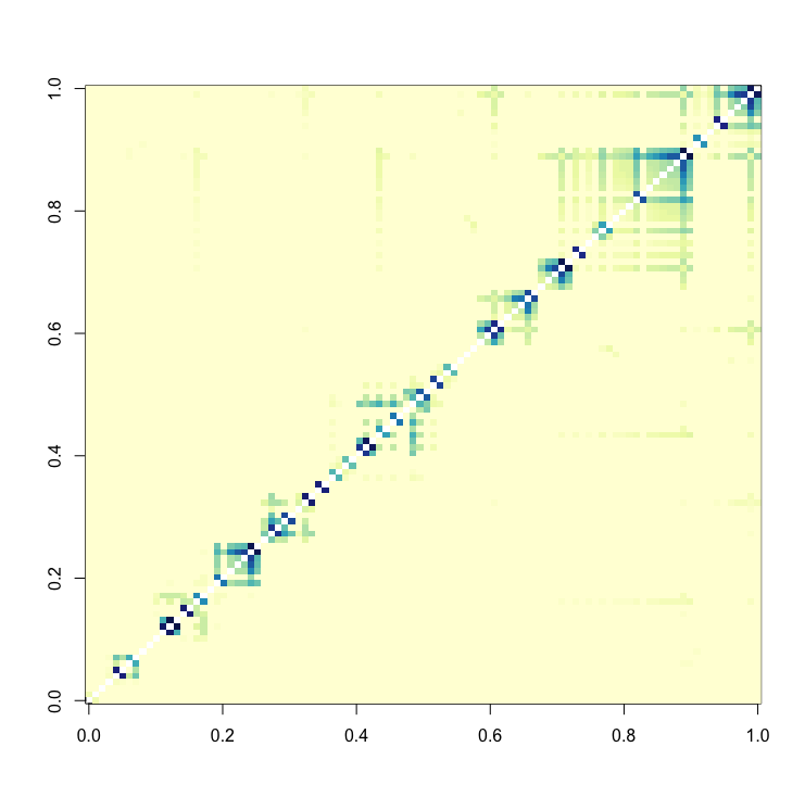
Visualize the matrix to get an overview of the topology:

image(wTO_matrix[node_order,node_order], useRaster=T, col=colorRampPalette(brewer.pal(9,"YlGnBu"))(49))

It is clear from the visualization that the network does not contain modular strucutres. However, we can observe highly connected nodes, i.e. hubs.

Tutorial part B: Locating protein complexes and bow-tie motifs

Since the toy network in part A do not contain modular structures, we load an adjacency matrix of the cDC1 cell, which is included in the bowtie R package. We will use only a subset of it in this tutorial.

data(cDC1_adj_matrix)
cDC1_adj_matrix_sub = cDC1_adj_matrix[400:600, 400:600]

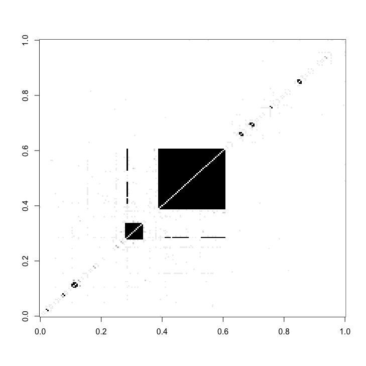
We locate the protein complexes in the adjacency matrix.

protein_complex_areas    = find_complexes(full_matrix = cDC1_adj_matrix_sub)
protein_complexes_merged = merge_complexes(protein_complex_areas)

We can highlight the areas that we have marked as protein complexes with red (lower matrix).

quick_matrix  = matrix(nrow = dim(cDC1_adj_matrix_sub)[1], ncol = dim(cDC1_adj_matrix_sub)[1], data = 0)

for (i in protein_complexes_merged){
  start = head(i, n=1)
  end   = tail(i, n=1)
  quick_matrix[start:end, start:end] = 2
}

quick_matrix[upper.tri(quick_matrix)] = cDC1_adj_matrix_sub[upper.tri(cDC1_adj_matrix_sub)]
grey_scale                            = colorRampPalette(brewer.pal(9,"Greys"))(21)

par(bg="white")
image(quick_matrix, useRaster = T,  col = c(grey_scale, 'red'), breaks = c(seq(0,1,0.05), 1.01, 2))

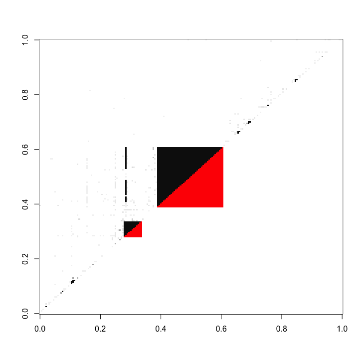
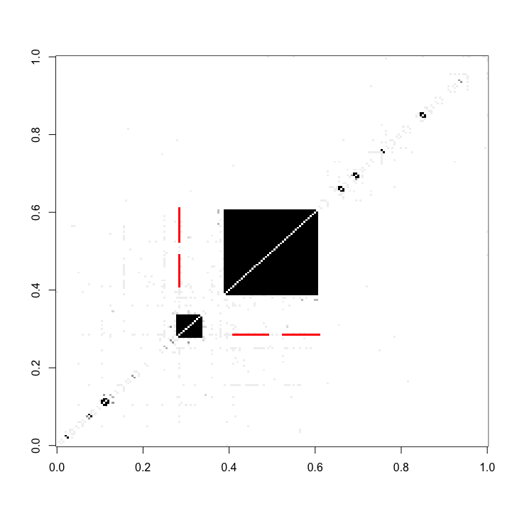
We then locate the bow-tie motifs in the adjacency matrix.

knot_proteins_and_fans = find_bowties(full_matrix = cDC1_adj_matrix_sub, protein_complex_areas = protein_complexes_merged)

The bow-tie interactions fans can also be visualized as red areas within the adjacency matrix.

int_matrix_combi = cDC1_adj_matrix_sub
for (knot_protein in names(knot_proteins_and_fans)){
  list_of_interaction_fans = knot_proteins_and_fans[[knot_protein]]
  
  for (interaction_fan in list_of_interaction_fans){
    index_ran                                 = interaction_fan[1]:interaction_fan[2]
    int_matrix_combi[knot_protein, index_ran] = 1.5
    int_matrix_combi[index_ran, knot_protein] = 1.5
  }
}

par(bg="white")
col_scale   = c(colorRampPalette(brewer.pal(9, 'Greys'))(10), 'red')
image(data.matrix(int_matrix_combi), useRaster=T, col = col_scale, breaks = c(seq(0, 1, 0.1), 2))

Authors

• PhD Student Kristoffer Niss - Coding and conceptual work
• Professor Søren Brunak - Conceptual work and supervision

Affiliation

Translational Disease Systems Biology Group, Novo Nordisk Foundation center for Protein Research (CPR), University of Copenhagen, 2200 Copenhagen, Denmark.

Publication

This R package is not published yet.

License

This project is licensed under the MIT License - see the LICENSE.md file for details

Acknowledgments

• Thank you to Tibor Varga and Grigorii Nos for help with setting up the R package