Four adversarial image crafting algorithms are implemented with Tensorflow.
The four attacking algorithms can be found in attacks folder. The
implementation adheres to the principle tensor-in, tensor-out. They all
return a Tensorflow operation which could be run through sess.run(...).
-
Fast Gradient Sign Method (FGSM) basic/iterative
fgsm(model, x, eps=0.01, epochs=1, clip_min=0.0, clip_max=1.0)
-
Target class Gradient Sign Method (TGSM)
tgsm(model, x, y=None, eps=0.01, epochs=1, clip_min=0.0, clip_max=1.0)
- When
y=None, this implements the least-likely class method. - If
yis an integer or a list of integers, the source image is modified towards labely.
- When
-
Jacobian-based Saliency Map Approach (JSMA)
jsma(model, x, y, epochs=1.0, eps=1., clip_min=0.0, clip_max=1.0, pair=False, min_proba=0.0)
yis the target label, could be an integer or a list. whenepochsis a floating number in the range[0, 1], it denotes the maximum percentage distortion allowed andepochsis automatically deduced.min_probadenotes the minimum confidence of target image. Ifpair=True, then modifies two pixels at a time. -
Saliency map difference approach (SMDA)
smda(model, x, y, epochs=1.0, eps=1., clip_min=0.0, clip_max=1.0, min_proba=0.0)
Interface is the same as
jsma. This algorithm differs from the JSMA in how the saliency score is calculated. In JSMA, saliency score is calculated asdt/dx * (-do/dx), while in SMDA, the saliency score isdt/dx - do/dx, thus the name "saliency map difference".
- Python3, samples codes uses many of the Python3 features.
- Numpy, only needed in sample codes.
- Tensorflow, tested with Tensorflow 1.1 and 1.3. Since there is no change in the API (only minor version number change), it should work with other versions as well.
Notice that we have model as the first parameter for every method. The
model is a wrapper function. It should have the following signature
def model(x, logits=False):
  # x is the input to the network, usually a tensorflow placeholder
  ybar = ...                    # get the prediction
  logits_ = ...                 # get the logits before softmax
  if logits:
    return y, logits
  return y
We need the logits because some algorithms (FGSM and TGSM) rely on the logits to compute the loss.
Implementation of each attacking method is self-contained, and depends only on
tensorflow. Copy the attacking method file to the same folder as your source
code and import it.
The implementation should work on any framework that is compatible with Tensorflow. I provide example code for Tensorflow and Keras in the folder tf_example and keras_example, respectively. Each code example is also self-contained.
And example code with the same file name implements the same function. For example, tf_example/ex_00.py and keras_example/ex_00.py implement exactly the same function, the only difference is that the former uses pure Tensorflow while the latter is built upon Keras.
-
ex_00.py trains a simple CNN on MNIST. Then craft adversarial samples from test data vis FGSM. The original label for the following digits are 0 through 9 originally, and the predicted label with probability are shown below each digit.
-
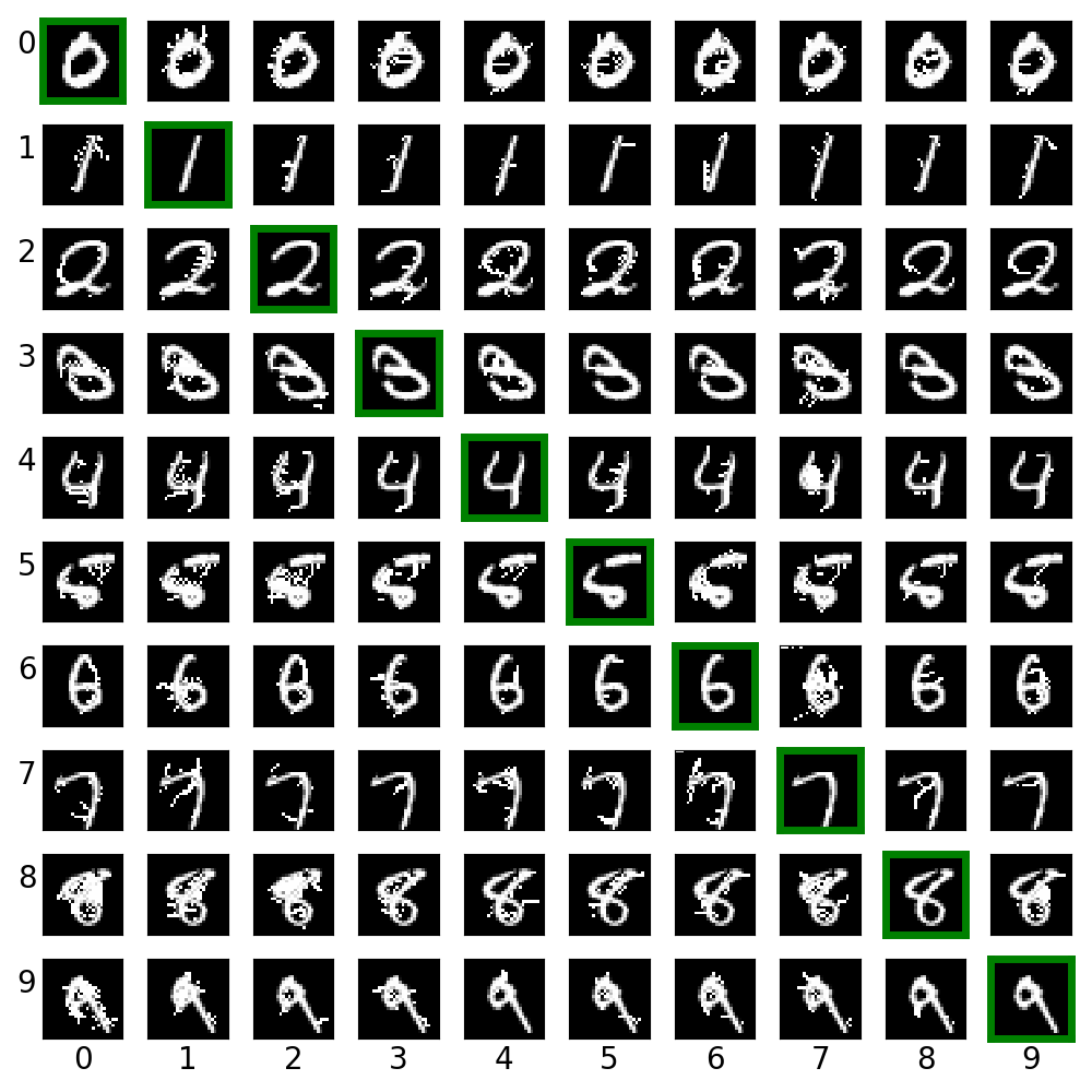
ex_01.py creates cross label adversarial images via saliency map approach (JSMA). For each row, the digit in green box is the clean image. Other images on the same row are created from it.
-
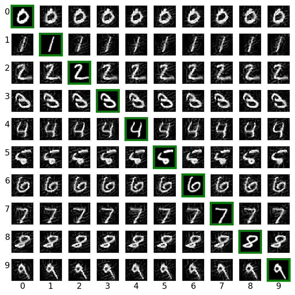
ex_02.py creates cross label adversarial images via target class gradient sign method (TGSM).
-
ex_03.py creates digits from blank images via saliency different algorithm (SMDA).
-
ex_04.py creates digits from blank images via paired saliency map algorithm, i.e., modify two pixels at one time (refer to the original paper for rational http://arxiv.org/abs/1511.07528).
These images look weird. And I have no idea why I could not reproduce the result in the original paper. My guess is that1. either my model is too simple to catch the features of the dataset, or2. there is a flaw in my implementation.However various experiments seem to suggest that my implementation work properly. I have to try more examples to figure out what is going wrong here.As suggested by Nicolas, I run JSMA for fixed epochs, and I could reproduce the images in his original paper. So it seems my JSMA implementation is correct.
-
ex_05.py trains a simple CNN on MNIST and then crafts adversarial samples via LLCM. The original label for the following digits are 0 through 9 originally, and the predicted label with probability are shown below each digit.
-
ex_06.py trains a CNN on CIFAR10 and then crafts adversarial image via FGSM.
- Update code with newer API from TensorFlow v1.3
- Add ImageNet examples
- Add attack method from https://arxiv.org/abs/1507.00677
- Add attack method from https://arxiv.org/abs/1608.04644
- Add houdini attack from https://arxiv.org/abs/1707.05373
- Add benchmark for various defense methods. There are so many of them, probably need a good survey, e.g. https://arxiv.org/abs/1705.07263.
- openai/cleverhans
- A list of related papers could be found RELATED.md.


