capGemContest: A Jupyter Notebook repository from kapilkd13

CapGemini DataScience Contest

Directory Structure

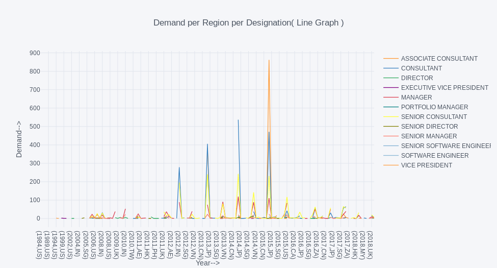
Jupyter notebook is present in Notebooks Folder
Data is in .csv format is present in Data Folder
Graph png's are present in Graph folder
Video demostration/Presentation is present in Video Folder. You can also download video from Google Drive: https://drive.google.com/file/d/1iiT-s3CqZ6mdOpcRQQvgxK44uQv_TgOf/view?usp=sharing
Predicted result is present in Result Folder. Its column structure is as follows:
1 Index: Month of the year
2 Demand: Predicted by model
3 optimal_demand: Optimized Demand after taking attrition and other factors
4 shifted_supply_2_month: Supply to hire in this month to met demand of 2 month in future.( It is just shifted demand by two months)( based on Task 2)

Key Instructions

Since the Jupyter Notebook Contains Interactive Graphs, it has been hosted here . For a non interactive version go here
Please have a look at the Presentation video, it's a bit long but it explains all the thought process, ideas, assumtions, results and will give you a complete tour of the jupyter notebook. Download the video from here
All three Tasks has been implemented inside Jupyter Notebook, i.e A prediction Model, A interactive cell where you can change values of variables like attrition, cost_per_resource etc. and see its affect on result and the predicted Supply for 2month advance, i.e S(N)=D(N+2)

Libraries

import numpy as np
import pandas as pd
import seaborn as sns
import json
import matplotlib.pyplot as plt
import sklearn
from sklearn.metrics import *
import math
import statsmodels.api as sm
from statsmodels.tsa.api import ExponentialSmoothing
from statsmodels.tsa.holtwinters import Holt
import cufflinks as cf
import plotly.plotly as py
import plotly.graph_objs as go

Apart from usual ML stack libraries, we used seaborn, plotly, cufflinks for plotting.
other ML model libraries includes statsmodels

Model Used

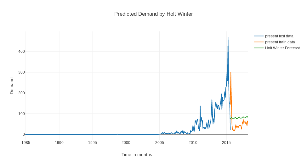
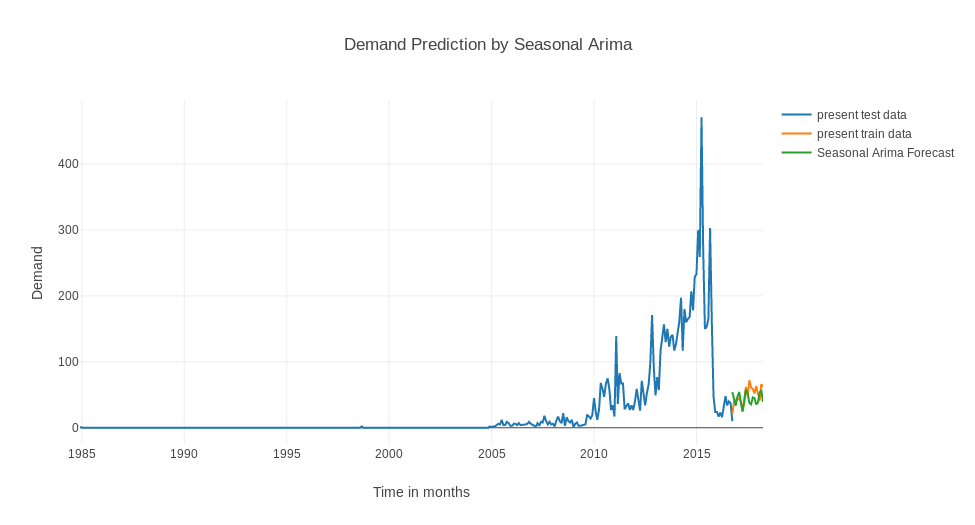
We comapred Result of Multiple models like Moving Average, Holt's Linear, Holt's Winter and ARIMA and Deasonal ARIMA. Finally we settled on Seasonal ARIMA.

Model Performance on Test set

RMSE( root mean square error)

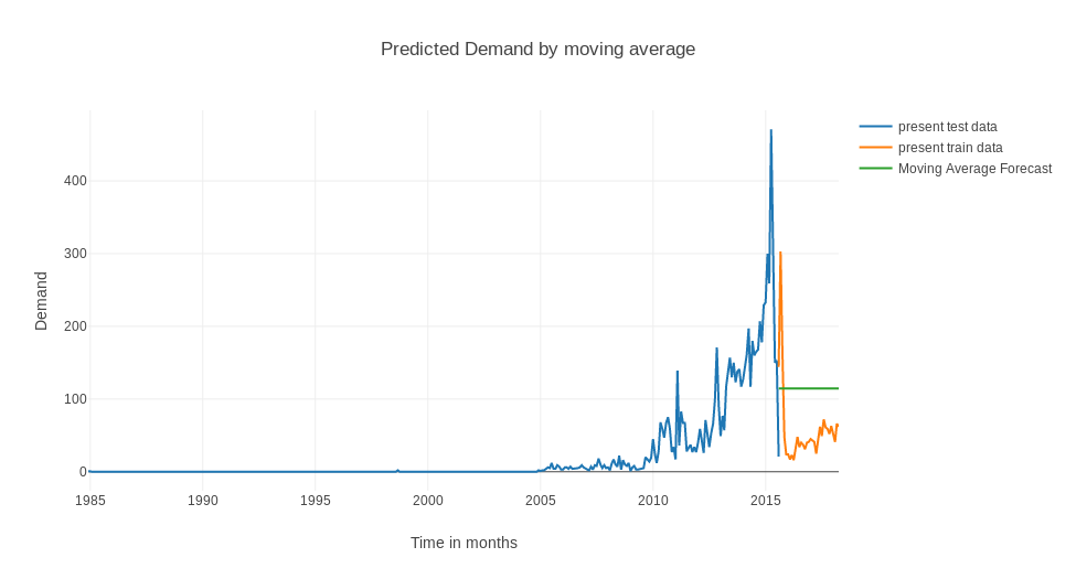
Moving average -- 70.1242656402115
Holt Linear -- 146.06096582776428
Holt Winter method -- 29.015957296157453
Seasonal Arima model -- 16.430577078652995

We decided to use Seasonal ARIMA model based on results.

Verification Instructions

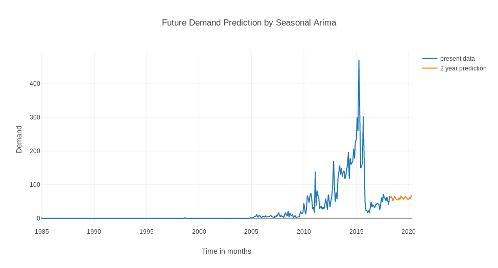
To verify these results, execute the jupyter Notebook. Notebook contains certain Notes on the selection of models, their results and other thoughts. The Video Presentation contains interactive flow through the complete Jupyter Notebook.

Final Thoughts

SARIMA model performed best of all the other model. Taking this as the base model, we can move forward with more advanced prediction like Demand per region per designation. This will allow us to predict more accurately.

kapilkd13/capGemContest