GeoTree: nearest-neighbors on geographic coordinates

Installation and setup
Tutorials
Tree build and query times, comparison between KDTree and BallTree

Installation

install using pip

pip install git+https://github.com/kasra-hosseini/geotree.git

install geotree from the source code:

Clone geotree source code:

git clone https://github.com/kasra-hosseini/geotree.git

Install geotree:

cd /path/to/my/geotree
pip install -v -e .

Alternatively:

cd /path/to/my/geotree
python setup.py install

Tutorials

Find closest neighbors (KDTree and BallTree)

⚠️ Jupyter notebook

Instantiate gtree:

from geotree import gtree
import matplotlib.pyplot as plt
import numpy as np

mytree = gtree()

Define the first set of points or base:

npoints = 200
lons = np.random.randint(-180, 180, npoints)
lats = np.random.randint(-90, 90, npoints)
depths = np.zeros(npoints)

Add lons/lats/depths of the first set of points:

mytree.add_lonlatdep(lons=lons, 
                     lats=lats, 
                     depths=depths)

⚠️ NOTE: depth is specified with respect to the Earth surface and in meters. Its axis points towards the center of the Earth, that is, positive depths specify points inside the Earth. Negative depths specify points above the Earth surface.

⚠️ In the above example, we used add_lonlatdep. For KDTree, these values are converted into x/y/z (Cartesian coordinate system) internally (and in meters). If you already have x/y/z in meters, you can use add_xyz function.

Define queries:

q_npoints = 10
q_lons = np.random.randint(-150, 150, q_npoints)
q_lats = np.random.randint(-70, 70, q_npoints)
q_depths = np.zeros(q_npoints)

Add lons/lats/depths of queries:

mytree.add_lonlatdep_query(lons=q_lons, 
                           lats=q_lats, 
                           depths=q_depths)

⚠️ In the above example, we used add_lonlatdep_query. For KDTree, these values are converted into x/y/z (Cartesian coordinate system) internally (and in meters). If you already have x/y/z in meters, you can use add_xyz_q function.

Find neighbors, kdtree:

Create KDTree (kdt):

mytree.create_kdt()

Choose the desired number of neighbors (and upper bound for distance, if needed):

mytree.query_kdt(num_neighs=3, distance_upper=np.inf)

Now, for each query, distances to the closest base neighbors and their indices are stored in (row-wise):

# distances to the closest `base` neighbors
mytree.dists2query

# indices of the closest `base` neighbors
mytree.indxs2query

The results are shown in the following figure. The base points are shown in black dots and the queries are shown by X. The closest three base neighbors are connected to each query.

Same results but on a interrupted Goode homolosine projection:

Find neighbors, Ball tree:

Create Ball tree:

mytree.create_balltree()

Choose the desired number of neighbors:

mytree.query_balltree(num_neighs=3)

Now, for each query, distances to the closest base neighbors and their indices are stored in (row-wise):

# distances to the closest `base` neighbors
mytree.dists2query

# indices of the closest `base` neighbors
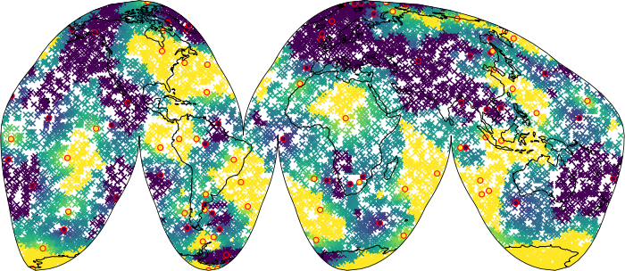
mytree.indxs2query

Interpolate values of one grid into another one

⚠️ Jupyter notebook

Here, we have a set of points, labelled as base in the figure below, with some values (i.e., colors of those points). We also have another set of points, queries in the figure, for which we want to compute values using the values of base. Geotree uses the following algorithm for this task:

it creates a tree (KDTree or BallTree) for base points.
for a query point, it finds the closest neighbors from base (the number of neighbors is specified by the user, in the figure below, this number was 4).
it assigns a value to the query point by computing the weighted average of the values of the neighboring base points. The weights are proportional to the inverse distance.

(See more results below)

Instantiate gtree:

from geotree import gtree
import numpy as np

mytree = gtree()

Define the first set of points or base:

npoints = 100
lons = np.random.randint(-180, 180, npoints)
lats = np.random.randint(-90, 90, npoints)
depths = np.zeros(npoints)

# assign some values (to each point)
vals = np.zeros(npoints)
vals[:(npoints//2)] = 0
vals[(npoints//2):] = 1

Add lons/lats/depths of the first set of points:

mytree.add_lonlatdep(lons=lons, 
                     lats=lats, 
                     depths=depths)

Define queries:

q_npoints = 10000
q_lons = np.random.randint(-180, 180, q_npoints)
q_lats = np.random.randint(-90, 90, q_npoints)
q_depths = np.zeros(q_npoints)

Add lons/lats/depths of queries:

mytree.add_lonlatdep_query(lons=q_lons, 
                           lats=q_lats, 
                           depths=q_depths)

Assign values to the first set of points: (note: size of vals should be the same as the first set of points)

mytree.add_vals(vals)

Interpolation: compute the values of queries from the values of base points:

KDTree

As the first example, we consider one neighbor (i.e., only the value of the closest base point to a query is used)

mytree.interpolate(num_neighs=1, method="kdtree")

mytree.interpolate(num_neighs=2, method="kdtree")

Or on a interrupted Goode homolosine projection:

mytree.interpolate(num_neighs=10, method="kdtree")

BallTree

In the above examples, we used KDTree, we can change the method to Ball tree by simply:

mytree.interpolate(num_neighs=2, method="balltree")

To plot the above figures:

import matplotlib.pyplot as plt
plt.figure(figsize=(15, 7))
plt.scatter(q_lons, q_lats, 
            c=mytree.interp_vals, 
            marker="x", 
            vmin=min(vals), vmax=max(vals),
            label="queries")

plt.scatter(lons, lats,
            c=vals, 
            marker="o",
            vmin=min(vals), vmax=max(vals), edgecolors="r",
            label="base",
            zorder=100)

plt.legend(bbox_to_anchor=(0., 1.01, 1., .05), 
           loc="right", ncol=2, 
           fontsize=16,
           borderaxespad=0.)

plt.title(f"Method: {mytree.interp_method}", size=16)
plt.colorbar()
plt.grid()
plt.tight_layout()
plt.show()

Conversion between lon/lat/depth and x/y/z

⚠️ Jupyter notebook

geotree can read lon/lat/depth or x/y/z as inputs. Here is a list of relevant functions:

add_lonlatdep (depth should be in meters; positive depths specify points inside the Earth.)
add_lonlatdep_query (same as above except for queries)
add_xyz (in meters)
add_xyz_q (for queries, in meters)

In this section, we show two functions in geotree: lonlatdep2xyz_spherical and xyz2lonlatdep_spherical. These are used internally to convert between lon/lat/dep and x/y/z.

from geotree import convert as geoconvert
import matplotlib.pyplot as plt
import numpy as np

Define a set of lons/lats/depths:

npoints = 100
lons = np.random.randint(-180, 180, npoints)
lats = np.random.randint(-90, 90, npoints)
depths = np.zeros(npoints)

lons/lats/depths ---> x/y/z

Here, we use geoconvert.lonlatdep2xyz_spherical to convert lons/lats/depths ---> x/y/z (in meters)

⚠️ We set depths to zeros, i.e., all points are on a sphere with a radius of 6371000 meters.

x, y, z = geoconvert.lonlatdep2xyz_spherical(lons, 
                                             lats, 
                                             depths, 
                                             return_one_arr=False)

In the figure:

Left pabel: in geographic coordinate
Right panel: x/y/z in meters (on a sphere with radius of 6371000m)

To plot the above figure:

fig = plt.figure(figsize=(12, 5))

plt.subplot(1, 2, 1)

plt.scatter(lons, lats,
            c="k", 
            marker="o",
            zorder=100)

plt.xlabel("lons", size=20)
plt.ylabel("lats", size=20)
plt.xticks(size=14); plt.yticks(size=14)
plt.xlim(-180, 180); plt.ylim(-90, 90)
plt.grid()

# ---
ax = fig.add_subplot(1, 2, 2, projection='3d')

ax.scatter3D(x, y, z, c="k", marker="o");

ax.set_xlabel('X (m)', size=16)
ax.set_ylabel('Y (m)', size=16)
ax.set_zlabel('Z (m)', size=16)

plt.tight_layout()
plt.show()

x/y/z ---> lons/lats/depths

Just as test, we now use geoconvert.xyz2lonlatdep_spherical to convert x/y/z back to lons/lats/depths:

lons_conv, lats_conv, depths_conv = geoconvert.xyz2lonlatdep_spherical(x, y, z, 
                                                                       return_one_arr=False)

and, we measure the L1 error between original lons/lats/depths and the ones computed above:

print(max(abs(lons - lons_conv)))
print(max(abs(lats - lats_conv)))
print(max(abs(depths - depths_conv)))

Outputs:

2.842170943040401e-14
2.842170943040401e-14
9.313225746154785e-10

Tree build and query times, comparison

⚠️ Jupyter notebook

The figure compares KDTree and Ball tree for build (left) and query (right) times. The left panel shows the build time as a function of number of points used in the tree. The build times of the two methods are very similar. In the right panel, we first constructed a tree for one million points and then measured the time to query this tree with different number of queries (x-axis).

See this Jupyter notebook for details.

kasra-hosseini/geotree

GeoTree: nearest-neighbors on geographic coordinates

Table of contents

Installation

Tutorials

Find closest neighbors (KDTree and BallTree)

Find neighbors, kdtree:

Find neighbors, Ball tree:

Interpolate values of one grid into another one

KDTree

BallTree

Conversion between lon/lat/depth and x/y/z

lons/lats/depths ---> x/y/z

x/y/z ---> lons/lats/depths

Tree build and query times, comparison