We are using a dataset related to ASHRAE – Great Energy Predictor III (How much energy will a building consume?) which is a competition in Kaggle you can refer to it here. The goal is to develop models from ASHRAE’s 2016 data in order to better understand metered building energy usage in the following areas: chilled water, electric, hot water, and steam meters. The data comes from over 1,000 buildings over a one-year timeframe.
The dataset includes three years of hourly meter readings from over one thousand buildings at several sites around the world. It contains some measurements and buildings information that could help for the building the model. You can refer here to learn more about dataset.
for the reason we deal with massive data, it is a well common fact to reduce the memory usage:

for example lets take the building_meta
site_id           0
building_id       0
primary_use       0
square_feet       0
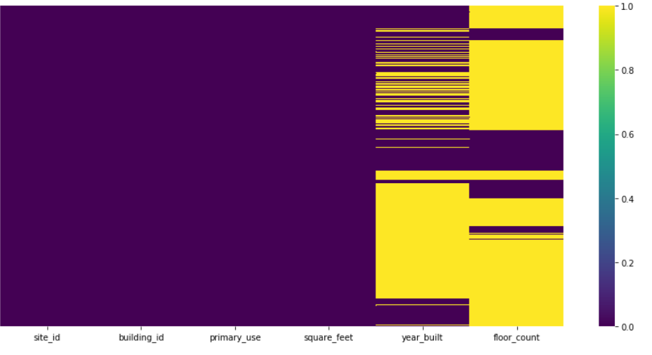
year_built      774
floor_count    1094
dtype: int64
this image illustrates these messing data with a heatmap plot:
Merging the data in one dataframe called BTW_train:
BuildingTrain = building_meta.merge(ASHRAE_train, left_on='building_id', right_on='building_id' , how='left')
BTW_train=BuildingTrain.merge(weather_train,left_on=['site_id','timestamp'],right_on=['site_id','timestamp'],how='left')
and then sorting this dataframe by the meter type , building_id, primary_use, Month and Day:
BTW_train= BTW_train.groupby(['meter',BTW_train['building_id'],'primary_use',BTW_train['Month'], BTW_train['Day']]).agg({'meter_reading':'sum', 'air_temperature': 'mean', 'wind_speed': 'mean', 'precip_depth_1_hr': 'mean', 'cloud_coverage': 'mean', 'square_feet': 'mean'})
After preparing the data with the process described above, we should fill the missing value :
BTW_train['precip_depth_1_hr'].fillna(method='ffill', inplace = True)
BTW_train['cloud_coverage'].fillna(method='bfill', inplace = True)

BTW_train['wind_speed'].fillna(BTW_train['wind_speed'].mean(), inplace=True)
BTW_train['air_temperature'].fillna(BTW_train['air_temperature'].mean(), inplace=True
To solve this problem, We crate a DeepLearning model based on LSTM units. This image below will illustrate our model architecture:
Model: "sequential_5"
_________________________________________________________________
Layer (type)                 Output Shape              Param #
=================================================================
lstm_9 (LSTM)                (None, None, 128)         71168
_________________________________________________________________
batch_normalization_9 (Batch (None, None, 128)         512
_________________________________________________________________
dropout_9 (Dropout)          (None, None, 128)         0
_________________________________________________________________
lstm_10 (LSTM)               (None, 128)               131584
_________________________________________________________________
batch_normalization_10 (Batc (None, 128)               512
_________________________________________________________________
dropout_10 (Dropout)         (None, 128)               0
_________________________________________________________________
dense_7 (Dense)              (None, 1)                 129
=================================================================
Total params: 203,905
Trainable params: 203,393
Non-trainable params: 512
_________________________________________________________________
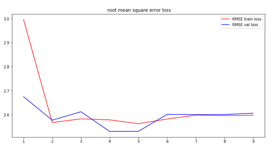
For the metric we use Root Mean Square Error as it is required in the competition. This type of error was manually added :
def root_mean_squared_error(y_true, y_pred):
  return K.sqrt(K.mean(K.square(y_pred - y_true)))
For the purpose of catching the best model behavior, we used the early stop method to detect the best time to stop the train before it went for worse.
es = EarlyStopping(monitor='val_root_mean_squared_error', min_delta=0.0001, patience=5, verbose=True, mode='auto')
Finally, this figure bellow will show you how the model perform:

