Lecture: Ultrafast dynamics

Jupyter notebooks for the lecture using numerical concepts for propagtion of physical systems in time and calculation of eigenenergiesm and other expectation values.

Required packages:

All notebooks are tested under the following package-versions:

Package	Version
python	3.9
numpy	1.22.2
scipy	1.7.3
matplotlib	3.3.4
ipython	7.30.1
ipympl	0.2.1

Hydrogen atom

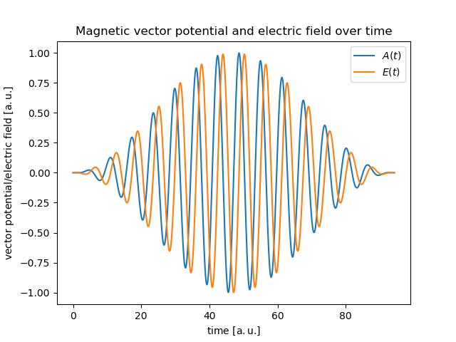
Propagation of atomic wavefunctions using the Multiphoton-Matrix-Iterative-Method on non-uniform grids. We use atomic units. The Hamiltonian reads

$$ \hat{H}0\Psi{\ell}(r, t)Y_{\ell,m}(\theta,\varphi) = \left(-\frac{1}{2 r^2}\frac{\partial}{\partial r}\left(r^2 \frac{\partial}{\partial r} \Psi_{\ell}(r, t) \right) + \frac{\ell(\ell+1)}{2r^2}\Psi_{\ell}(r, t) - \frac{1}{r}\Psi_{\ell}(r, t)\right) Y_{\ell,m}(\theta,\varphi).$$

High harmonic generation (HHG)

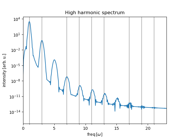
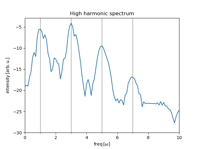
Artificial one-dimensional atom of the form $$\hat{H} = \frac{1}{2}\hat{p}^2 + \hat{V}(\hat{x}) + E_0 \hat{x} f(t) \cos(\omega t),$$ where $f(t)$ is the envelope function of a $\sin^2-!$ laser pulse. We choose Dirichlet boundary conditions, $\psi(x_{\text{min}})=0$ and $\psi(x_{\text{max}})=0$.

Two-level system

Generic two-level system subjected to an external classical field is described via the Hamiltonian

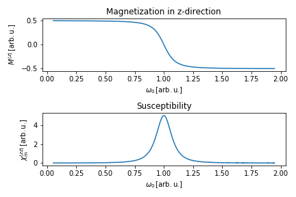
$$\hat{H}=\frac{\omega_0}{2} \hat{\sigma}_z + \frac{B_0}{2} ( \hat{\sigma}_x \cos(\omega t) + \hat{\sigma}_y \sin(\omega t)).$$

Calculations of various expectation values like magnetization and susceptibility $$M^{(z)} \sim \partial E / \partial \omega_0,$$ $$\chi_{\mathrm{m}}^{(zz)} \sim \partial^2 E / \partial \omega_0^2.$$

Tight-Binding models