FFT

傅里叶分解

1. Modeling

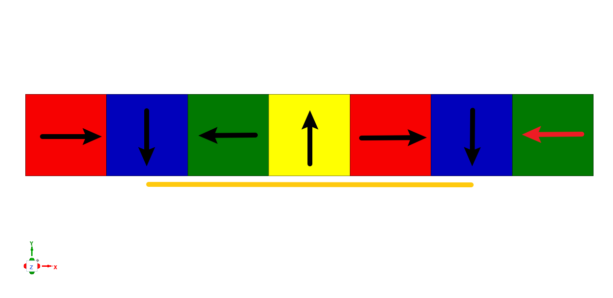
The magnetization directions of the PMs based on the Halbach linear motor are shown in the figure below,

2. FFT by Maxwell

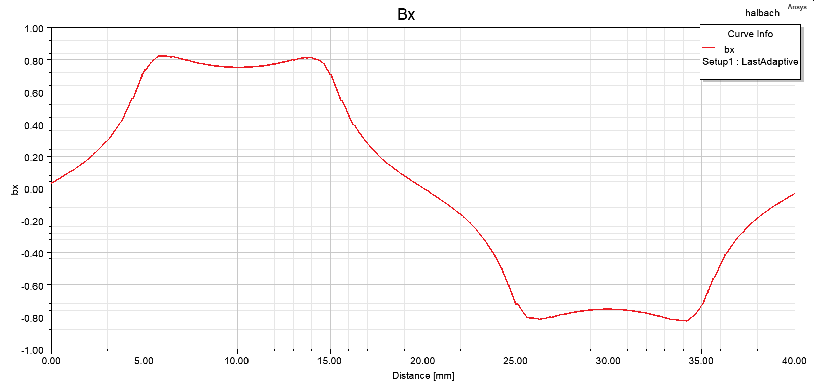
The magnetic density waveform of the air-gap under a pair of poles is obtained by Maxwell as shown in the figure below,

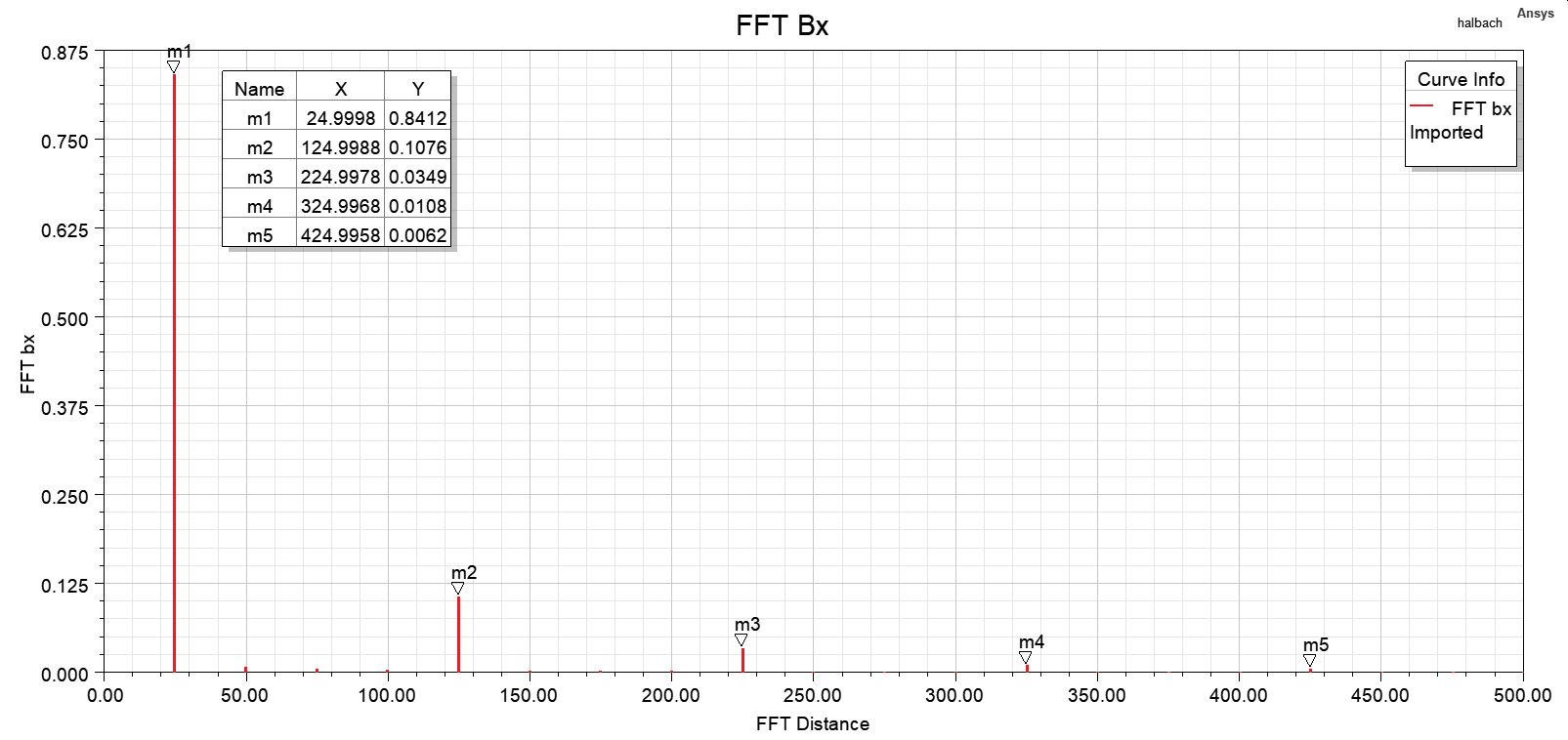
The Fourier decomposition is obtained by maxwell's FFT as shown in the figure below,

3. FFT by python & Matplotlib (Recommended)

Export the air-gap magnetic density ($B_x$) to csv format and the FFT code in python is as follows,

import numpy as np
import pandas as pd
import matplotlib.pyplot as plt
from matplotlib.pylab import mpl
 
mpl.rcParams['font.sans-serif'] = ['SimSun']
mpl.rcParams['axes.unicode_minus']=False
#plt.rcParams['figure.dpi'] = 300
plt.rcParams['figure.constrained_layout.use'] = True

fig = plt.figure()
fixed_width_mm = 340
fixed_height_mm = 170
fixed_width_inch = fixed_width_mm / 25.4
fixed_height_inch = fixed_height_mm / 25.4
fig.set_size_inches(fixed_width_inch, fixed_height_inch)

ax1 = fig.add_subplot(121)
ax2 = fig.add_subplot(122)

data = pd.read_csv('Bx.csv')
x = data['Distance [mm]']
y = data['bx []']
ax1.plot(x,y,color='r',label='orgin',ls='--')

fft_y=np.fft.fft(y)
N=fft_y.shape[0]

orders=11
order=orders+1

fundamental=np.abs(fft_y[1])/N*2
harmonics=np.abs(fft_y[2:order])/N*2
thd=np.sqrt(np.sum(harmonics**2))/fundamental
thd_per = round(thd*100, 2)

for i in range(order):
	new_fft_y=np.zeros_like(fft_y)
	new_fft_y[i]=fft_y[i]
	ifft_y=np.fft.ifft(new_fft_y).real*2
	ax1.plot(x,ifft_y,label='order='+str(i))
	normalization_y=np.abs([fft_y[i]])/N*2
	ax2.bar(i,normalization_y)

ax1.legend()
ax1.set_title('各次谐波分解示意图')
ax1.set_xlabel('长度(mm)')
ax1.set_ylabel('各次谐波幅值大小')
ax1.set_xlim(x[0],x[len(x)-1])

ax2.set_title('各次谐波FFT分解柱状图 (THD='+str(thd_per)+'%)')
ax2.set_xlabel('谐波次数')
ax2.set_ylabel('各次谐波幅值大小')
ax2.set_xlim(0,order)
ax2.set_xticks(np.arange(0,order,1))

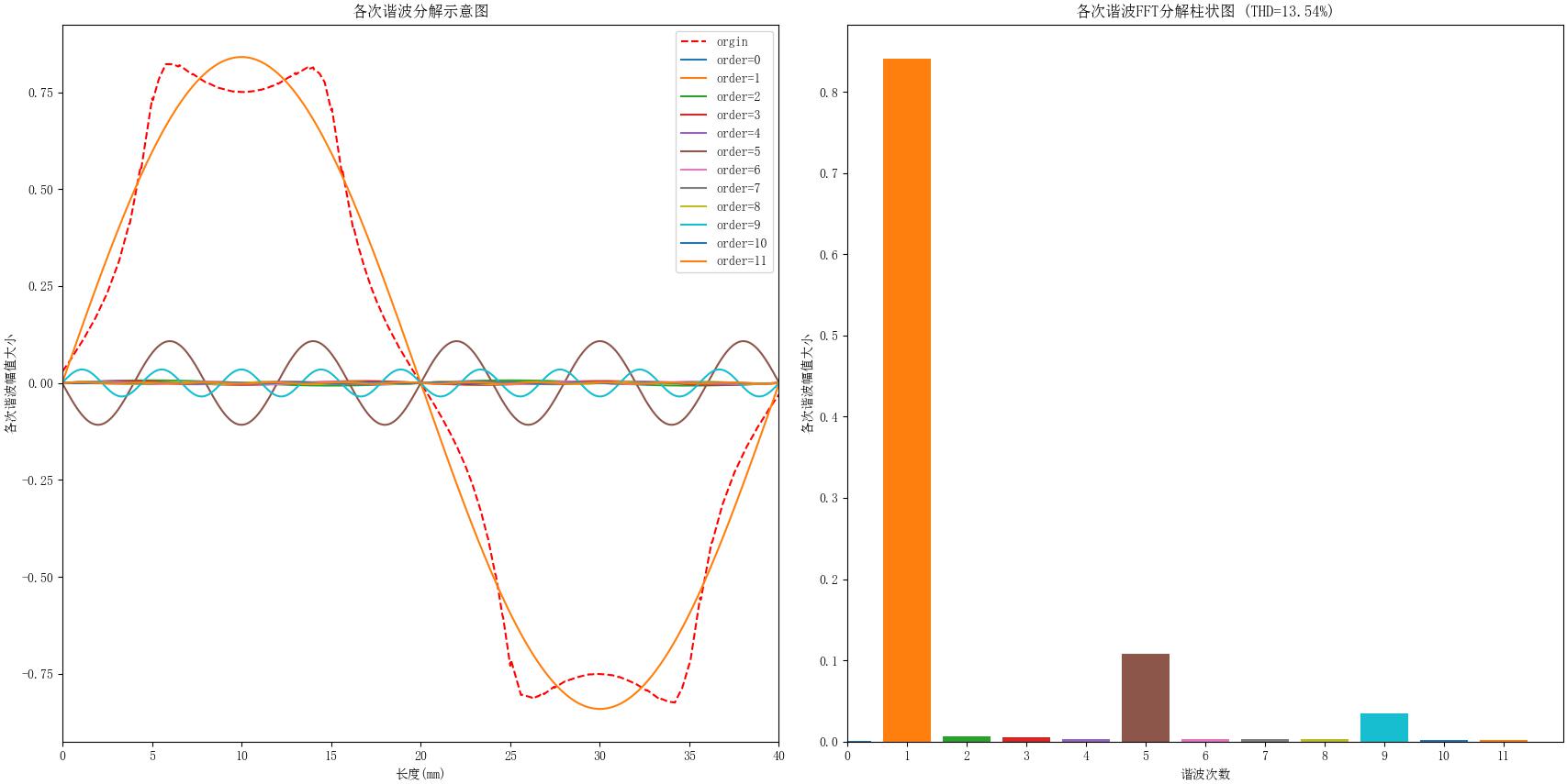
plt.show()

The FFT is as follows,

4. FFT by Matlab (Not recommended)

Export the air-gap magnetic density ($B_x$) to csv format and the FFT code in matlab is as follows,

clc
clear all;
format long;
Ns=1001;		%采样点
order=11;		%谐波数
filename='Bx.csv';		%导出的气隙磁密数据集
data=csvread(filename,1,0);     %从行偏移量 R1 和列偏移量 C1 开始读取文件中的数据
x=data(:,1);        %取第一列
y=data(:,2);        %取第二列
figure;
plot(x,y,'r');      %plot origional waveform
hold on;
grid on;
fft1=fft(y,Ns);
j=0;
amp_har=zeros(1,(order));
%%
for m=1:1:order
j=j+1;
fft1=fft(y,Ns);
fund_ele_front=fft1(m+1);
fund_ele_back=fft1(Ns+1-m);
amp_har(j)=(abs(fund_ele_front))/Ns*2;
fft1=0*fft1;
fft1(m+1)=fund_ele_front;
fft1(Ns+1-m)=fund_ele_back;
fft1=ifft(fft1,Ns);
fft1=real(fft1);
plot(x,fft1);
title('各次谐波分解示意图')
xlabel('长度(mm)')
ylabel('各次谐波幅值大小')
hold on;
end
%%
k=(1:1:order);
figure;
bar(k,amp_har);
title('各次谐波FFT分解柱状图')
xlabel('谐波次数')
ylabel('各次谐波幅值大小')
grid on;
peak_b=max(fft1);
rms_b=0.707*peak_b;
s=amp_har.^2;
THD = sqrt(sum(s(2:(order+1)/2)))/(amp_har(1));
THD_pct = 100*THD;

The decomposition of each harmonic is as follows,

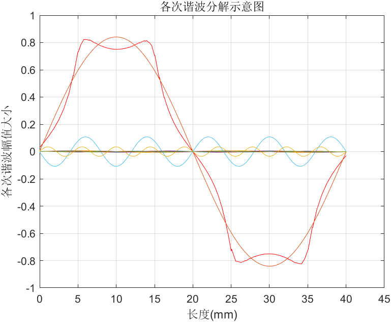
The histogram of FFT decomposition of each harmonic is as follows,

About Project

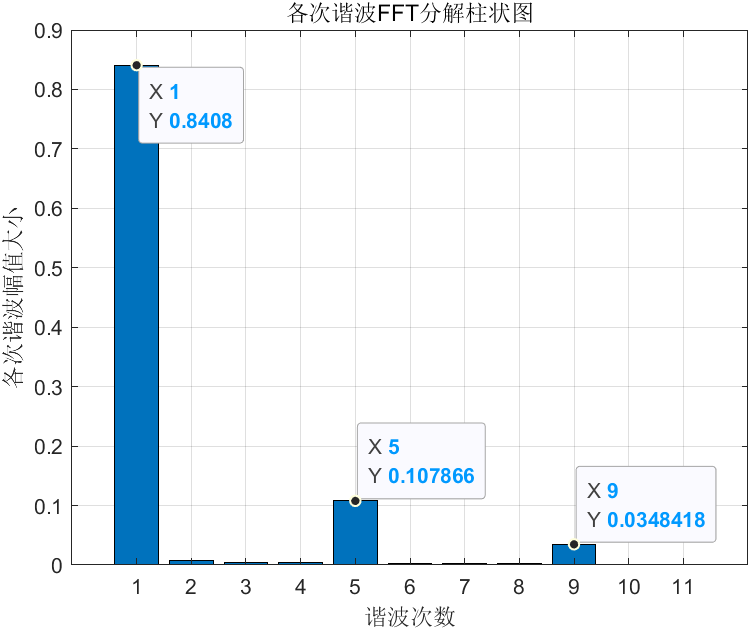
Version：ANASYS Electronics Suite 2021 R2