An R package for Grade of Membership (GoM) model fit and visualization of counts data.
Kushal K Dey, Chiaowen Joyce Hsiao, Matthew Stephens
IMPORTANT UPDATE: We encourage CountClust users to use our new R package, fastTopics. This new package has most of CountClust's features, plus several important improvements, including model fitting algorithms that are faster and more accurate.
If you are find CountClust useful, please cite:
Dey K, Hsiao C, and Stephens M (2017). Visualizing the structure of RNA-seq expression data using grade of membership models. PLoS Genetics 13: e1006599
Taddy M (2012). On Estimation and Selection for Topic Models. AISTATS, JMLR 22.
CountClust requires the following CRAN-R packages: slam, ggplot2, cowplot, parallel along with the Bioconductor package: limma.
One can install CountClust from Bioc as follows
source("http://bioconductor.org/biocLite.R")
biocLite("CountClust")
For installing the working version of this package from Github please run
install_github('kkdey/CountClust')
To avoid bug issues for large datasets, we recommend the user to install the latest maptpx package from Github.
library(devtools)
install_github('TaddyLab/maptpx')
To replicate the data example in this README, please install the following data package.
install_github('kkdey/singleCellRNASeqMouseDeng2014')
Then load the CountClust package in R:
library(CountClust)
We load the single cell RNA-seq data due to Deng et al 2014. The data contains RNA-seq read counts for single cells at different stages of mouse embryo development (from zygote to blastocyst).
library(singleCellRNASeqMouseDeng2014)
deng.counts <- exprs(Deng2014MouseESC)
deng.meta_data <- pData(Deng2014MouseESC)
deng.gene_names <- rownames(deng.counts)
We apply the FitGoM function (which is a wrapper of the topics function in the maptpx package) for a user specified number of clusters (K=6 for the example below).
FitGoM(t(deng.counts),K=3,path_rda="data/MouseDeng2014.FitGoM.rda")
This function will output a list - of which the key components are the two matrices omega and theta. omega denotes the matrix of cluster memberships for each sample and theta denotes the matrix of proportional contribution of each feature to a cluster.
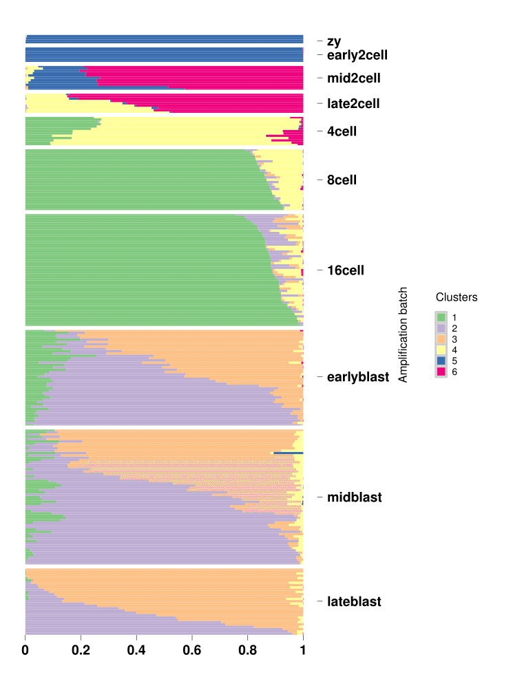
One can plot the omega from the FitGoM functionusing a Structure Bar plot. Here we provide an example of the Structure plot for K=6 for the above GoM model fit.
data("MouseDeng2014.FitGoM")
names(MouseDeng2014.FitGoM)
omega <- MouseDeng2014.FitGoM$clust_6$omega


annotation <- data.frame(
  sample_id = paste0("X", c(1:NROW(omega))),
  tissue_label = factor(rownames(omega),
                        levels = rev( c("zy", "early2cell",
                                        "mid2cell", "late2cell",
                                        "4cell", "8cell", "16cell",
                                        "earlyblast","midblast",
                                         "lateblast") ) ) )

rownames(omega) <- annotation$sample_id;

StructureGGplot(omega = omega,
                annotation = annotation,
                palette = RColorBrewer::brewer.pal(8, "Accent"),
                yaxis_label = "Amplification batch",
                order_sample = TRUE,
                axis_tick = list(axis_ticks_length = .1,
                                 axis_ticks_lwd_y = .1,
                                 axis_ticks_lwd_x = .1,
                                 axis_label_size = 7,
                                 axis_label_face = "bold"))
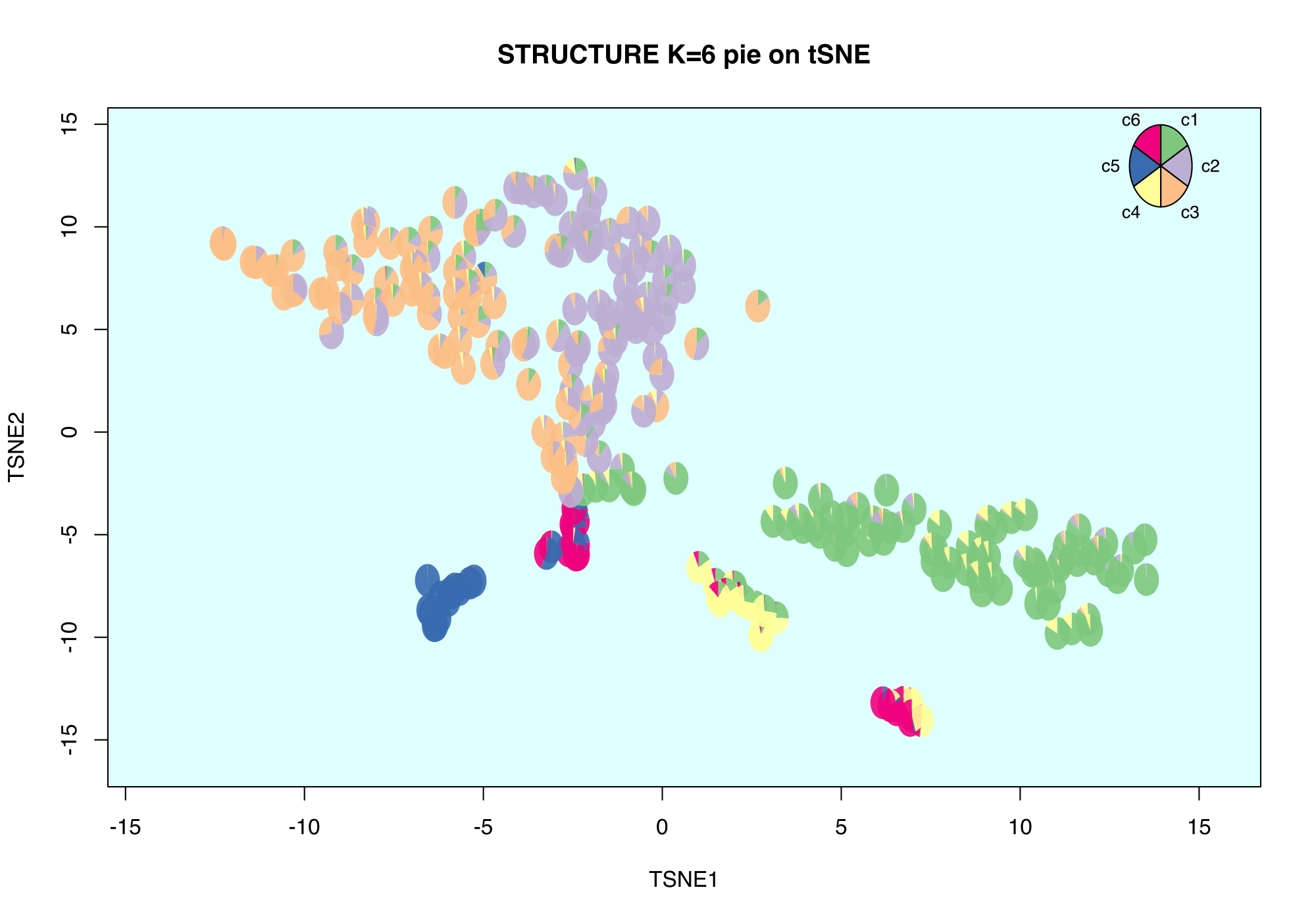
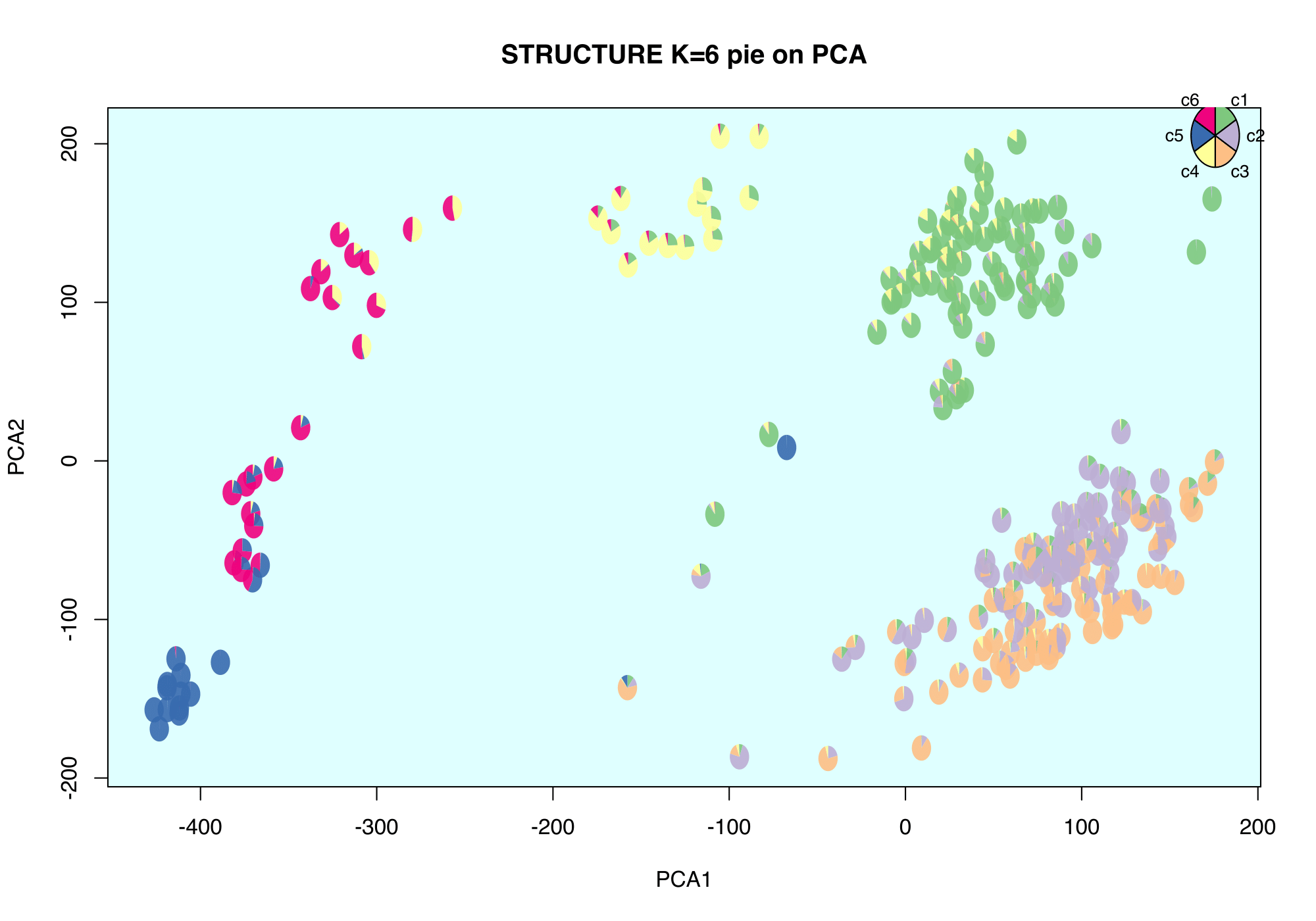
One can also visualize the STRUCTURE grades of membership colorings aggregated with the t-SNE or the PCA plots, as follows.
t-SNE + CountClust grades coloring
StructurePie(t(deng.counts), input_type="apply_tsne",
             use_voom=FALSE, omega = omega, xlab="TSNE1",
             ylab = "TSNE2",
             main = "STRUCTURE K=6 pie on tSNE",
             control = list(bg = "lightcyan"))
PCA + CountClust grades coloring
StructurePie(t(deng.counts), input_type="apply_pca",
             use_voom = TRUE, omega = omega, xlab="PCA1",
             ylab = "PCA2",
             main = "STRUCTURE K=6 pie on PCA",
             control = list(bg = "lightcyan"))
We can extract the features that drive the clusters for K=6 as follows
theta_mat <- MouseDeng2014.topicFit$clust_6$theta;
top_features <- ExtractTopFeatures(theta_mat, top_features=100,
                                   method="poisson", options="min");
gene_list <- do.call(rbind, lapply(1:dim(top_features)[1],
                        function(x) deng.gene_names[top_features[x,]]))
It will provide you with a list of top 100 variables/features per cluster that are relatively most highly expressed in that cluster compared to the other clusters, or in other words, plays the most important role in driving or separating out that cluster from the rest.
The CountClust package is distributed under [GPL - General Public License (>= 2)]
For any questions or comments, please contact kkdey@uchicago.edu
- Raman Shah
- Peter Carbonetto


