Languages and libraries used:
- Pandas
- Numpy
- Matplotlib
- SQLAlchemy
- DateTime
- Flask
- JSON
-
Jupyter notebook,
climate.ipynband hawaii.sqlite files were used to complete the climate analysis and data exploration. -
SQLAlchemy
create_engineconnects to the sqlite database. -
SQLAlchemy
automap_base()reflects the tables into classes and saves a reference to those classes calledStationandMeasurement. -
Linked Python to the database by creating an SQLAlchemy session.
-
Found the most recent date in the data set.
- Most recent date: 2017, 08, 23
-
Used this date to retrieve the last 12 months of precipitation data by querying the 12 preceding months of data.
- Selected only the
dateandprcpvalues.
- Selected only the
-
Loaded the query results into a Pandas DataFrame and set the index to the date column.
-
Sorted the DataFrame values by
date. -
Plotted the results using the DataFrame
plotmethod.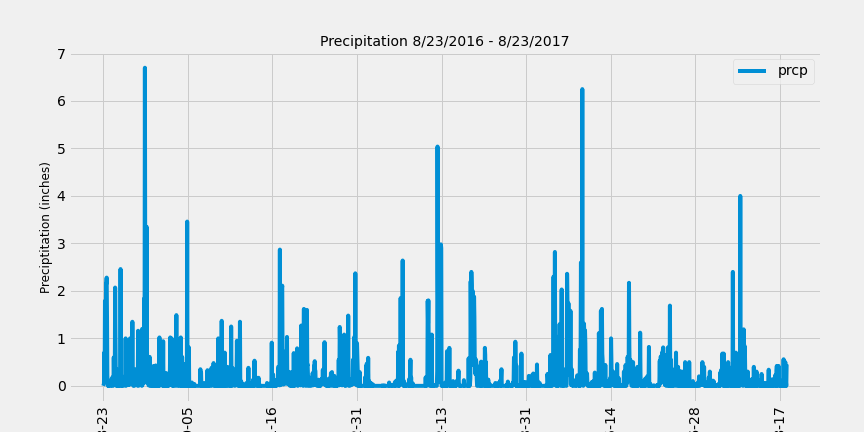
-
Used Pandas to print the summary statistics for the precipitation data.
count 2021.000000
mean 0.177279
std 0.461190
min 0.000000
25% 0.000000
50% 0.020000
75% 0.130000
max 6.700000

-
Queried to calculate the total number of stations in the dataset.
-
Queried to find the most active stations.
-
Listed the stations and observation counts in descending order.
-
Determined which station id had the highest number of observations.
- Station with most observations: USC00519281
-
Used the most active station id, calculated the lowest, highest, and average temperature.
count 352.000000
mean 73.107955
std 4.733315
min 59.000000
25% 70.000000
50% 74.000000
75% 77.000000
max 83.000000
-
-
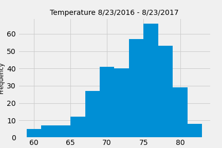
Queried to retrieve the last 12 months of temperature observation data (TOBS).
-
Filtered by the station with the highest number of observations.
-
Queried the last 12 months of temperature observation data for this station.
-
Plotted the results as a histogram with
bins=12.
-

Designed a Flask API based on the previously developed queries.
- Used Flask to create routes.
-
/Home page-
Available Hawaii API Routes:
- /api/v1.0/precipitation
- /api/v1.0/stations
- /api/v1.0/tobs
- /api/v1.0/<start>
- /api/v1.0/<start>/<end>
- /api/v1.0/precipitation
-
-
/api/v1.0/stations-
Converted the query results to a dictionary using
dateas the key andprcpas the value. -
Returned the JSON representation of the dictionary.
-
-
/api/v1.0/stations- Returned a JSON list of stations from the dataset.
-
/api/v1.0/tobs-
Queried the dates and temperature observations of the most active station for the last year of data.
-
Returned a JSON list of temperature observations (TOBS) for the previous year.
-
-
/api/v1.0/<start>and/api/v1.0/<start>/<end>-
Returned a JSON list of the minimum temperature, the average temperature, and the max temperature for a given start or start-end range.
-
With the start only, calculated
TMIN,TAVG, andTMAXfor all dates greater than and equal to the start date. -
With the start and the end date, calculated the
TMIN,TAVG, andTMAXfor dates between the start and end date inclusive.
-
-
Determined if there is a meaningful difference between the temperature in June and December in Hawaii.
-
Identified the average temperature in June and December at all stations across all available years in the dataset.
- June: 74.94411764705882
- December: 71.04152933421226
-
An independent t-test was performed to determine whether the difference in the means, if any, is statistically significant.
-
Ttest_indResult(statistic=31.60372399000329, pvalue=3.9025129038616655e-191)
-
Null Hypothesis: Temperatures in Hawaii in June and December have no statistically significant difference.
-
Reject the Null Hypothesis
-
There is a statistically significant difference in the temperatures in June and December in Hawaii.
-
-
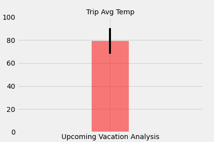
Used historical data in the dataset find out what the temperature had previously looked like.
-
Used the
calc_tempsfunction to calculate the min, avg, and max temperatures for the trip using the matching dates from a previous year. -
Plotted the min, avg, and max temperature as a bar chart.
-
Used the average temperature as the bar height (y value).
-
Used the peak-to-peak (TMAX-TMIN) value as the y error bar (YERR).
-

-
Used historical data in the dataset to find out what the precipitation had previously looked like
-
Calculated the rainfall per weather station using the previous year's dates (i.e. "2017-08-01").
- Sorted in descending order by precipitation amount and list the station, name, latitude, longitude, and elevation.
-
-
Calculated the daily normals. Normals are the averages for the min, avg, and max.
-
Set the start and end date of the trip.
- Used the date to create a range of dates.
-
Removed the year and saved a list of strings in the format
%m-%d. -
Use the
daily_normalsfunction to calculate the normals for each date string and append the results to a list.
-
-
Loaded the list of daily normals into a Pandas DataFrame and set the index equal to the date.
-
Used Pandas to plot an area plot for the daily normals.
