binfer

This package aims to make doing Bayesian things a little easier by giving a clear set of steps that you can easily use to simulate draws from a posterior distribution defined by a specific likelihood and prior.

The steps

define a likelihood

Input: A data frame, a formula with the response variable and the name of a function that is your likelihood.
Output: A data frame with the name of the function given at input as an attribute

assume a prior distribution

Input: A data frame and a function of a single variable
Ouput: A data frame with the name of the function added as an attribute

draw from the posterior distribution

Input: A data frame, a control parameter
Output: A data frame of draws from the posterior distribution

diagnose the chain:

Input: a data frame of draws from the posterior
Output: The same data frame and a bunch of diagnostic plots

clean the chain

Input: Draws from the posterior
Output: Burned-in and subsampled draws from the posterior

Construct your confidence interval or p-value

Use dplyr for this

Examples

Estimate the standard deviation of a normal distribution with a gamma prior:

library(binfer)
library(tidyverse)
#> Loading tidyverse: ggplot2
#> Loading tidyverse: tibble
#> Loading tidyverse: tidyr
#> Loading tidyverse: readr
#> Loading tidyverse: purrr
#> Loading tidyverse: dplyr
#> Warning: package 'tibble' was built under R version 3.4.3
#> Conflicts with tidy packages ----------------------------------------------
#> filter(): dplyr, stats
#> lag():    dplyr, stats

my_lik <- function(data, theta) {if (theta > 0) dnorm(data, mean = mean(iris$Sepal.Width) , sd = theta) else 0}
my_prior <- function(theta) {dgamma(theta, shape = 10, rate = 20)}

posterior <- define(iris, Sepal.Width ~ my_lik) %>% 
  assume(prior = ~ my_prior) %>% 
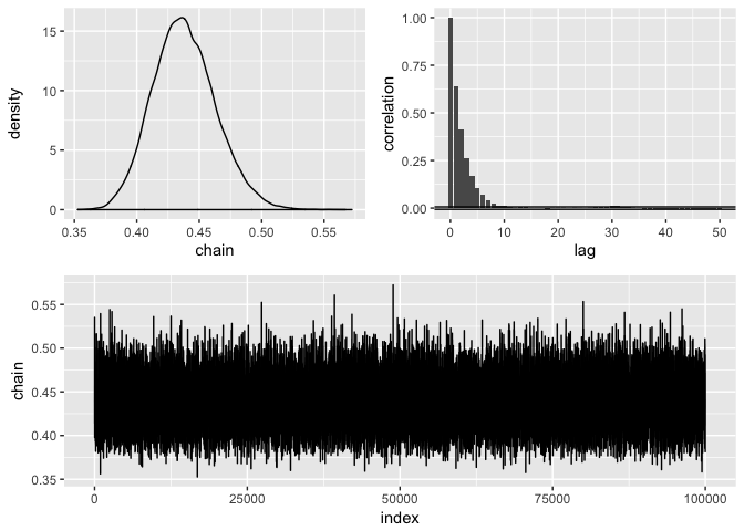
  draw(initial = .43, nbatch = 1e5, blen = 1, scale = .05) %>% 
  diagnose() %>% 
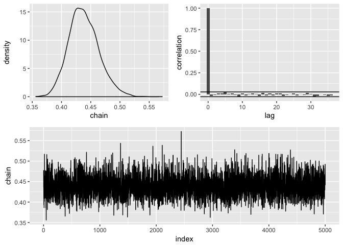
  clean(burnin = 0, subsample = 20) %>% 
  diagnose()
#> Acceptance rate: 0.497534975349753
#> Acceptance rate: 1

posterior %>% summarise(mean = mean(chain),
                        sd = sd(chain),
                        lower = quantile(chain, .025),
                        upper = quantile(chain, .975))
#>        mean         sd     lower    upper
#> 1 0.4382871 0.02558842 0.3925185 0.493049

Estimate the probability of success of a binomnial distribution with a beta prior and compare the analytical solution to the approximate one:

binom_test_data <- rbinom(50, prob = .1, size = 1) %>% 
  tibble(response = .)

binom_lik <- function(data, theta) {if(theta > 0 & theta < 1) dbinom(data, prob = theta, size = 1) else 0}
beta_prior <- function(theta) {dbeta(theta, 1, 2)}

posterior2 <- binom_test_data %>% 
  define(response ~ binom_lik) %>% 
  assume(~ beta_prior) %>% 
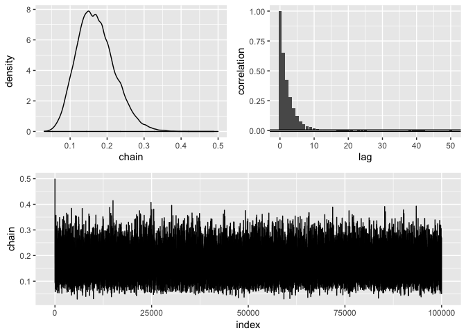
  draw(initial = .5, nbatch = 1e5, blen = 1, scale = .15) %>% 
  diagnose() %>% 
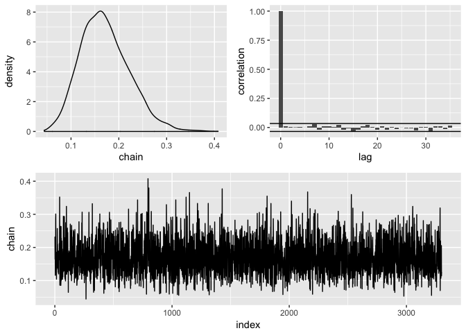
  clean(burnin = 1000, subsample = 30) %>% 
  diagnose()
#> Acceptance rate: 0.376063760637606
#> Acceptance rate: 1

posterior2 %>% 
  summarize(mean = mean(chain), 
            sd = sd(chain), 
            lower = quantile(chain, .025), 
            upper = quantile(chain, .975))
#> # A tibble: 1 x 4
#>    mean     sd  lower upper
#>   <dbl>  <dbl>  <dbl> <dbl>
#> 1 0.171 0.0508 0.0853 0.282

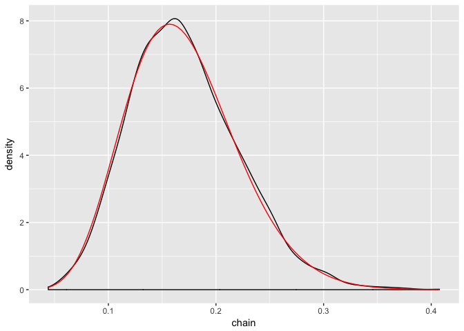
ggplot(posterior2, aes(chain)) + 
  geom_density() +
  stat_function(fun = dbeta, 
                args = list(1 + sum(binom_test_data$response), 
                            2 + nrow(binom_test_data) - sum(binom_test_data$response)),
                color = "red")

klmedeiros/binfer

binfer

The steps

Examples