klmr/minimappr

Code minimaps for R

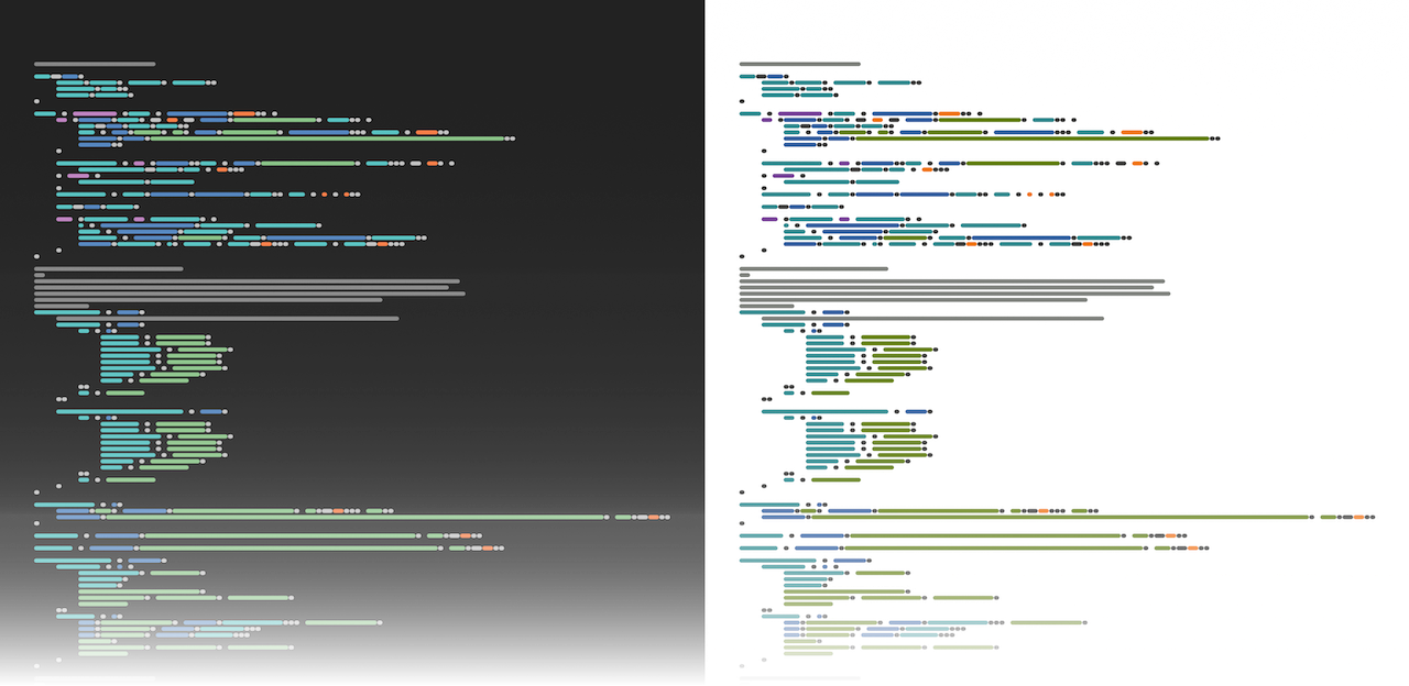
Code minimaps in R

Code minimaps are a feature of some modern code editors in which the code is displayed with a drastically reduced font size, so that all that can be discerned are patterns based on indentation, line length and syntax colouring.

Ostensibly code minimaps help navigating large files. Well, maybe. But when done right they become interesting design elements.

So how do we do it right? First of, rather than actually printing text I wanted to have plain lines (printing text makes the image much more visually busy, and looks messy). To plot lines from source code, we therefore need to obtain a tokenised representation of the source code with syntax information (for the colours) and somehow generate x/y coordinates for each token.

Luckily, R makes this much easier than is reasonable: when parsing source code (via parse), we can retain the internal parse data, and retrieve it in tabular form via getParseData:

expr = parse(text = '1 + 2', keep.source = TRUE)
getParseData(expr)

	line1	col1	line2	col2	id	parent	token	terminal	text
7	1	1	1	5	7	0	expr	FALSE
1	1	1	1	1	1	2	NUM_CONST	TRUE	1
2	1	1	1	1	2	7	expr	FALSE
3	1	3	1	3	3	7	'+'	TRUE	+
4	1	5	1	5	4	5	NUM_CONST	TRUE	2
5	1	5	1	5	5	7	expr	FALSE

This generates a lot of data that isn’t interesting for us: we only care about those pieces that are “terminals”:

box::use(dplyr[`%>%`, filter])

getParseData(expr) %>% filter(terminal)

line1	col1	line2	col2	id	parent	token	terminal	text
1	1	1	1	1	2	NUM_CONST	TRUE	1
1	3	1	3	3	7	'+'	TRUE	+
1	5	1	5	4	5	NUM_CONST	TRUE	2

And this is almost exactly what we need to pass it directly to ‘ggplot2’ (with the source code added as labels to clearly show what is being plotted):

box::use(ggplot2[...])

expr = parse(text = 'f = function () {\n    1 + 2\n}', keep.source = TRUE)

getParseData(expr) %>%
    filter(terminal) %>%
    ggplot() +
    aes(x = col1, y = line1, xend = col2 + 0.5, yend = line1, color = token) +
    geom_segment(size = 2) +
    geom_text(aes(label = text), hjust = 0, size = 4, color = 'black')

Hmm. OK, a few things:

1. The whole thing is on its head. To fix this, we need to specify scale_y_continuous(trans = 'reverse').
2. We probably want to remove the grid, axes and background. This means: theme_void().
3. Oh, and also the legend.
4. Rounded segments look better.

getParseData(expr) %>%
    filter(terminal) %>%
    ggplot() +
    aes(x = col1, y = line1, xend = col2 + 0.5, yend = line1, color = token) +
    geom_segment(size = 2, lineend = 'round') +
    scale_y_continuous(trans = 'reverse') +
    scale_color_discrete(guide = FALSE) +
    theme_void()

Much better, but there’s still room for improvement:

1. There are too many different token types (and, consequently, too many colours). To fix this, we need to replace, for instance, all the different punctuation tokens ('(', ')', '+', EQ_ASSIGN etc.) with a single token type.
2. The colours aren’t exactly pretty. Luckily, the internet is full of syntax highlighting colour schemes for us to choose from.
3. The spacing is off. This will require adding margins, and calculating suitable plot dimensions to fit the source code appropriately.
4. In the above I’ve added an offset of 0.5 to col2 so that tokens consisting of a single character are visible. But tokens adjacent to spaces look better if both their start and end are offset instead.

All this is implemented in the module minimap.r. This module generated the images at the beginning of the article.

The module requires ‘box’. It can be run either as a stand-alone command from the command line:

./minimap [-c colorscheme] input-file.r

… or it can be imported and used from other R code:

box::use(klmr/minimap)

filename = 'input-file.r'
p = minimap$plot_code_minimap(filename, minimap$colorschemes$tomorrow)
plot(p)
# To save the plot, calculate its ideal dimensions first:
dim = minimap$minimap_dim(filename)