Advanced Lane Finding Project
The goals / steps of this project are the following:
- Compute the camera calibration matrix and distortion coefficients given a set of chessboard images.
- Apply a distortion correction to raw images.
- Use color transforms, gradients, etc., to create a thresholded binary image.
- Apply a perspective transform to rectify binary image ("birds-eye view").
- Detect lane pixels and fit to find the lane boundary.
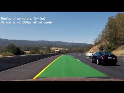
- Determine the curvature of the lane and vehicle position with respect to center.
- Warp the detected lane boundaries back onto the original image.
- Output visual display of the lane boundaries and numerical estimation of lane curvature and vehicle position.
Camera Calibration
The code for this step is contained in the first code cell of the Jupyter notebook located in "./project.ipynb".
I start by preparing "object points", which will be the (x, y, z) coordinates of the chessboard corners in the world. Here I am assuming the chessboard is fixed on the (x, y) plane at z=0, such that the object points are the same for each calibration image. Thus, objp is just a replicated array of coordinates, and objpoints will be appended with a copy of it every time I successfully detect all chessboard corners in a test image. imgpoints will be appended with the (x, y) pixel position of each of the corners in the image plane with each successful chessboard detection.
I then used the output objpoints and imgpoints to compute the camera calibration and distortion coefficients using the cv2.calibrateCamera() function.
The image looked like this before

I applied this distortion correction to the test image using the cv2.undistort() function and obtained this after

Pipeline (single images)
Step 1. Distortion-correction of images
Here we just apply the distortion-correction to any incoming images:

Step 2. Colour and gradients thresholded images
I used a combination of color and gradient thresholds to generate a binary image (In the "Spatial threshold functions" and "Colour threshold functions" cells of the IPython notebook). Here's an example of my output for this step.

Step 3. Perspective transform
The code for my perspective transform includes a function called warp(), (in the "Perspective Transform of region of interest" cell of the IPython notebook). The warp() function takes as inputs an image (img), as well as source (src) and destination (dst) points. I chose to hardcode the source and destination points by choosing the source and destination points from one of the still images of the road. This resulted in the following points:
| Source | Destination |
|---|---|
| 260, 680 | 260, 720 |
| 610, 450 | 260, 0 |
| 696, 450 | 1075, 0 |
| 1075, 671 | 1075, 720 |

Step 4. Finding the Lane Lines
Then I partisioned the image into 9 different horizontal slices and in each of these slices I would find the "best" point of the left and right lanes. Then with all of these point I fit two second degree polynomials to them. (in the "Finding the Lane Lines" cell of the IPython notebook)

Step 5. Radius of curvature
I did this in the "Measuring Curvature and Displacement" cell of the IPython notebook.
To figure out the position of the vehicle with respect to center of the lane I compared the center of the image to the midpoint of the left and right polynomials to get how many pixels the car was from the center then I converted the number of pixels to meters.
Step 6. End of the pipeline
I implemented this step in the "Transform Polynomial back to original image" cell of the IPython notebook using a function called transformPolyOnImg(). Here is an example of my result on a test image:

Pipeline (video)
Here is a link to see the pipline in action
Discussion
We could improve the prformance of the pipline when applied to videos from keeping track of where the estimations of the prevoius lanes are. The pipeline is likely to fail on dirt roads or possibly roads where the lane lines are very fated out.