Traffic Sign Recognition
The goals / steps of this project are the following:
- Load the data set (see below for links to the project data set)
- Explore, summarize and visualize the data set
- Design, train and test a model architecture
- Use the model to make predictions on new images
- Analyze the softmax probabilities of the new images
- Summarize the results with a written report
Writeup / README
You're reading it! and here is a link to my project code
Data Set Summary & Exploration
1. Basic summary of the data set
The code for this step is contained in the second code cell of the IPython notebook.
I used the numpy library to calculate summary statistics of the traffic signs data set:
- The size of training set is 34799
- The size of test set is 12630
- The shape of a traffic sign image is (32, 32, 3)
- The number of unique classes/labels in the data set is 43
2. Visualization of the dataset
The code for this step is contained in the third code cell of the IPython notebook.
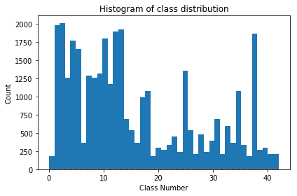
Here is an exploratory visualization of the data set. It is a bar chart showing the count of how many images we have of each class, we see that some classes how many more images some of the other
Design and Test a Model Architecture
1. Preprocessing the image data.
The code for this step is contained in the fifth code cell of the IPython notebook.
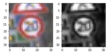
As a first step, I decided to convert the images to grayscale because since most of the perceived colour spectrum is contained in just the green and red channels. This also makes it easyer to train the model since it converting to grayscale removes having to learn a given sign in different lighting conditions (sunny vs cloudy). Then we preform a histogram equalization to make the images be in the range [0...1] so the optimizer can tone the model to find features more easily this way.
Here is an example of a traffic sign image before and after grayscaling.
2. Training, validation, and testing data.
The code for splitting the data into training and validation sets is contained in the first code cell of the IPython notebook since we were provided pickle files for the train, test and validation sets.
My final training set had 34799 number of images. My validation set and test set had 4410 and 12630 number of images.
3. Model architecture
The code for my final model is located in the seventh cell of the ipython notebook labeled "Final Tensorflow Model".
My final model consisted of the following layers:
| Layer | Description |
|---|---|
| Input | 32x32x1 Grayscale image |
| Convolution 5x5 | 1x1 stride, same padding, outputs 28x28x8 |
| Max pooling | 2x2 stride, outputs 14x14x8 |
| Dropout | .8875 dropout probability |
| RELU | |
| Convolution 3x3 | 1x1 stride, same padding, outputs 12x12x16 |
| Dropout | .8875 dropout probability |
| RELU | |
| Convolution 3x3 | 1x1 stride, same padding, outputs 10x10x32 |
| Dropout | .8875 dropout probability |
| RELU | |
| Flatten | output 3200 |
| RELU | |
| Fully connected | output 240 |
| Fully connected | output 43 |
| Softmax |
4. Trained the model.
The code for training the model is located in the eigth cell of the ipython notebook labeled.
To train the model, I used 50 Epochs with a batch size of 128. The learning rate that was used was 0.0008 with a adma optimizer combined with a loss function of softmax_cross_entropy_with_logits
The code for calculating the accuracy of the model is located in the ninth cell of the Ipython notebook.
My final model results were:
-
training set accuracy of 99.96%
-
validation set accuracy of 94.74%
-
test set accuracy of 92.75%
-
What was the first architecture that was tried and why was it chosen? The first architecture that as used was the LeNet architecture since LeNet can classify digits/symboles hence it should be extended to classify traffic signs since a lot of signs contain letters (other symboles) on them.
-
What were some problems with the initial architecture? Well intially LeNet can only classify 10 different classes.
-
How was the architecture adjusted and why was it adjusted? Typical adjustments could include choosing a different model architecture, adding or taking away layers (pooling, dropout, convolution, etc), using an activation function or changing the activation function. One common justification for adjusting an architecture would be due to over fitting or under fitting. A high accuracy on the training set but low accuracy on the validation set indicates over fitting; a low accuracy on both sets indicates under fitting. We added one more convolutional and fully connected layers as well as removing some of the max pooling infavor of adding dropouts, Since we have a larger number of classes to consider as well as this lead to better preformance of the model.
-
Which parameters were tuned? How were they adjusted and why? The learing rate and the dropout probability, batch size were tuned. For the learning rate originally we started with 0.001 and was we were traning we noticed that the accuracy was fluctuating so we would gradually decrease the learning to get better preformance. We pick the dropout rate by doing a binary search starting with 1.0 and 0.5 and found that 0.8875 worked well. We picked batch size as 128 since we thought it would have good hardware alignment.
-
What are some of the important design choices and why were they chosen? For example, why might a convolution layer work well with this problem? How might a dropout layer help with creating a successful model? convolution layer work well with this problem since the signs have spatial patterns that the convolutional layers can pick up. The dropouts make it so that the the high level features are not overly dependent on just one low level feature.
Test a Model on New Images
1. Testing on new data.
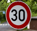
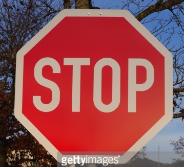
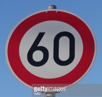
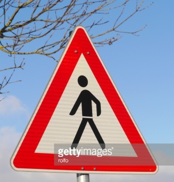
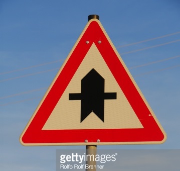
Here are five German traffic signs that I found on the web:
The classifier should be able to handle all of the above images. For the first three it should be easy to classify since there are a lot of traning examples of these classes. For the pedestrian image it might be a bit harder since there is a tree branches in the background. The last images should also be easy to classify.
2. Model's predictions the new data
The code for making predictions on my final model is located in the 13th cell of the Ipython notebook.
Here are the results of the prediction:
| Image | Prediction |
|---|---|
| 30 km/h | 30 km/h |
| Stop Sign | Stop sign |
| 60 km/h | 60 km/h |
| Pedestrians | Pedestrians |
| Right-of-way | Right-of-way |
The model was able to correctly guess 5 of the 5 traffic signs, which gives an accuracy of 100%. This compares so favorably to the accuracy on the test set.
3. Certain of the model
The code for making predictions on my final model is located in the 14th cell of the Ipython notebook.
For the first image, the model is absolutely sure that this is a 30 km/h sign ('probability' of 1.0), the image does contain a 30 km/h sign. The top five soft max probabilities were
| Probability | Prediction |
|---|---|
| 1.00000000e+00 | Speed limit (30km/h) |
| 2.19082197e-19 | Speed limit (20km/h) |
| 2.55120595e-21 | Speed limit (50km/h) |
| 8.04285170e-26 | End of speed limit (80km/h) |
| 7.68007737e-26 | Speed limit (70km/h) |
For the second image, the model is absolutely sure that this is a Stop sign ('probability' of 0.999), the image does contain a Stop sign. The top five soft max probabilities were
| Probability | Prediction |
|---|---|
| 9.99981761e-01 | Stop |
| 1.67283033e-05 | Wild animals crossing |
| 9.17447437e-07 | Speed limit (70km/h) |
| 4.32132140e-07 | Speed limit (30km/h) |
| 1.60738040e-07 | Speed limit (50km/h) |
For the third image, the model is absolutely sure that this is a 60 km/h ('probability' of 1.0), the image does contain a 60 km/h sign. The top five soft max probabilities were
| Probability | Prediction |
|---|---|
| 1.00000000e+00 | Speed limit (60km/h) |
| 3.08523731e-08 | Speed limit (50km/h) |
| 3.26723240e-14 | Speed limit (80km/h) |
| 1.58675563e-14 | Road work |
| 5.57797793e-15 | Keep right |
For the fourth image, the model is relatively sure that this is a Pedestrians sign ('probability' of 0.78), the image does contain a Pedestrians sign. The top five soft max probabilities were
| Probability | Prediction |
|---|---|
| 7.86758602e-01 | Pedestrians |
| 1.92155138e-01 | Right-of-way |
| 2.10388340e-02 | General caution |
| 4.73187974e-05 | Roundabout mandatory |
| 4.49821620e-08 | Dangerous curve to the right |
For the fifth image, the model is absolutely sure that this is a Right-of-way sign ('probability' of 0.999), the image does contain a Right-of-way sign. The top five soft max probabilities were
| Probability | Prediction |
|---|---|
| 9.99897599e-01 | Right-of-way |
| 1.02438862e-04 | Beware of ice/snow |
| 1.30390809e-08 | Slippery road |
| 1.39894110e-10 | Children crossing |
| 2.31572851e-11 | End of no passing by vehicles over 3.5 metric tons |
