{homophily}
They say that “birds of a feather flock together”, but why take their word for it?
Introduction
In social networks, actors tend to associate with others who are similar in some way, such as race, language, creed, or class. This phenomenon is called homophily.
The {homophily} package provides flexible routines to measure mixing
patterns using generic methods that are compatible with <network> and
<igraph> objects, including {tidygraph}’s <tbl_graph> objects.
Installation
# install.packages("remotes")
remotes::install_github("knapply/homophily")
Usage
library(homophily)data("jemmah_islamiyah", package = "homophily") # undirected <igraph>
data("sampson", package = "ergm") # directed <network>Mixing Matrices
We can easily build classical mixing matrices for undirected and directed graphs.
as_mixing_matrix(jemmah_islamiyah, dim1 = "role")#> 5 x 5 Matrix of class "dtrMatrix"
#>
#> command team operation assistant bomb maker suicide bomber Team Lima
#> command team 6 16 30 2 8
#> operation assistant . 2 10 2 0
#> bomb maker . . 20 10 0
#> suicide bomber . . . 0 8
#> Team Lima . . . . 12
as_mixing_matrix(samplike, dim1 = "group")#> 3 x 3 Matrix of class "dgeMatrix"
#>
#> Turks Outcasts Loyal
#> Turks 30 1 5
#> Outcasts 7 10 1
#> Loyal 9 2 23
Remixing Mixing Matrices
We can also build generalized mixing matrices to explore mixing patterns across different dimensions.
For example, if we want to explore ties between each individual node and
a group attribute, we can provide arguments to both dim1= and dim2=.
We’ll use the {network} convention of node names being stored in an
attribute called "vertex.names" to see mixing patterns between each
node and the "group" attribute.
as_mixing_matrix(samplike, dim1 = "vertex.names", dim2 = "group")#> 18 x 3 Matrix of class "dgeMatrix"
#>
#> Turks Outcasts Loyal
#> John Bosco 9 3 5
#> Gregory 11 3 1
#> Basil 3 5 0
#> Peter 0 0 9
#> Bonaventure 3 2 8
#> Berthold 1 0 5
#> Mark 8 2 1
#> Victor 4 0 7
#> Ambrose 2 0 6
#> Romauld 1 1 6
#> Louis 3 0 5
#> Winfrid 10 0 1
#> Amand 1 4 3
#> Hugh 8 0 3
#> Boniface 8 0 1
#> Albert 6 0 2
#> Elias 1 5 0
#> Simplicius 3 6 0
Going further, we can also explore mixing patterns across group
attributes. samplike’s "cloisterville" attribute notes whether each
individual attended the Cloisterville monastery.
as_mixing_matrix(samplike, dim1 = "cloisterville", dim2 = "group")#> 2 x 3 Matrix of class "dgeMatrix"
#>
#> Turks Outcasts Loyal
#> TRUE 34 15 24
#> FALSE 48 16 39
For directed graphs, the default behavior considers both outgoing and
inbound ties, but you can provide "out" or "in" to direction= as
desired.
as_mixing_matrix(samplike, dim1 = "cloisterville", dim2 = "group",
                 direction = "out")
#> 2 x 3 Matrix of class "dgeMatrix"
#>
#> Turks Outcasts Loyal
#> TRUE 15 5 10
#> FALSE 31 8 19
as_mixing_matrix(samplike, dim1 = "cloisterville", dim2 = "group",
                 direction = "in")
#> 3 x 2 Matrix of class "dgeMatrix"
#>
#> TRUE FALSE
#> Turks 19 17
#> Outcasts 10 8
#> Loyal 14 20
E-I Index
ei_index(jemmah_islamiyah, node_attr_name = "role")#> [1] 0.3650794
ei_index(jemmah_islamiyah, node_attr_name = "role", scope = "group")#> command team operation assistant bomb maker suicide bomber Team Lima
#> 0.8064516 0.7142857 -0.3333333 1.0000000 -1.0000000
ei_index(jemmah_islamiyah, node_attr_name = "role", scope = "node")#> MUKLAS AMROZI IMRON SAMUDRA DULMATIN IDRIS MUBAROK AZAHARI GHONI
#> 0.5555556 0.5000000 1.0000000 0.7333333 0.1111111 0.6000000 0.3333333 0.1111111 0.1111111
#> ARNASAN RAUF OCTAVIA HIDAYAT JUNAEDI PATEK FERI SARIJO
#> 1.0000000 -0.2000000 -0.2000000 -0.2000000 -0.2000000 0.1111111 1.0000000 0.1111111
ei_index(samplike, node_attr_name = "group")#> [1] -0.4318182
ei_index(samplike, node_attr_name = "group", scope = "group")#> Turks Outcasts Loyal
#> -0.6666667 -0.8181818 -1.0000000
ei_index(samplike, node_attr_name = "group", scope = "node")#> John Bosco Gregory Basil Peter Bonaventure Berthold Mark Victor
#> -0.05882353 -0.46666667 -0.25000000 -1.00000000 -0.23076923 -0.66666667 -0.45454545 -0.27272727
#> Ambrose Romauld Louis Winfrid Amand Hugh Boniface Albert
#> -0.50000000 -0.50000000 -0.25000000 -0.81818182 0.00000000 -0.45454545 -0.77777778 -0.50000000
#> Elias Simplicius
#> -0.66666667 -0.33333333
Assortativity
assort_discrete(jemmah_islamiyah, node_attr_name = "role")#> [1] 0.09078704
assort_discrete(samplike, node_attr_name = "group")#> [1] 0.5445606
assort_degree(samplike) #> [1] 0.05569702
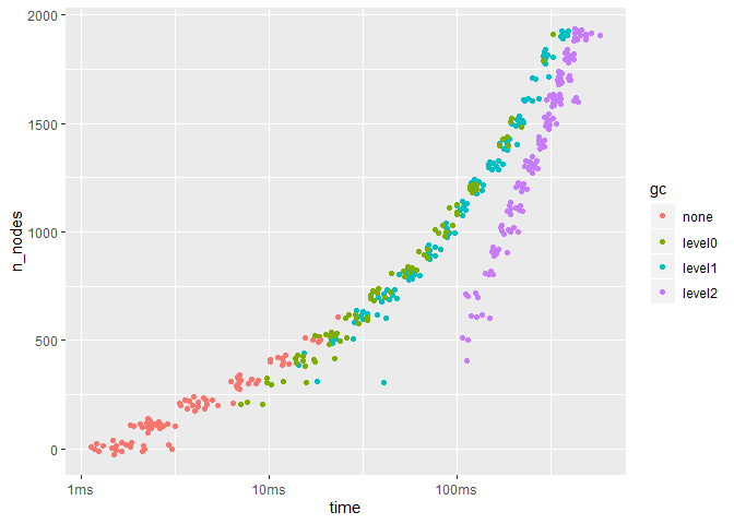
Benchmarks
library(tidyr)
library(bench)
library(ggplot2)
library(igraph)


build_it <- function(n_nodes, prob = 0.25, dir = TRUE) {
  g <- random.graph.game(n_nodes, prob, directed = dir)
  vertex_attr(g, name = "group") <- sample(letters, n_nodes, replace = TRUE)
  g
}

bench_it <- function(bench_foo, seq_nodes = seq(10, 2000, by = 100), ...) {
  all_res <- lapply(seq_nodes, function(x) {
    g <- build_it(x)
    res <- mark(
      bench_foo(build_it(x), node_attr_name = "group"),
      iterations = 20
    )
    res[["n_nodes"]] <- x
    res
  })
  do.call(rbind, all_res)
}set.seed(831)
res <- bench_it(ei_index)
res %>%
unnest() %>%
ggplot(aes(x = n_nodes, y = time)) +
ggbeeswarm::geom_quasirandom(aes(color = gc)) +
coord_flip()R CMD Check
devtools::check(quiet = TRUE)#> Writing NAMESPACE
#> Writing NAMESPACE
#> -- R CMD check results --------------------------------------------------- homophily 0.0.0.9000 ----
#> Duration: 34.9s
#>
#> 0 errors v | 0 warnings v | 0 notes v
Cite
citation("homophily")#>
#> To cite homophily use:
#>
#> Knapp, B. G. (2019). homophily: Measuring Network Homophily Data. R package version
#> 0.0.0.9 Retrieved from https://knapply.github.io/homophily
#>
#> A BibTeX entry for LaTeX users is
#>
#> @Manual{homophily-package,
#> title = {homophily: Measuring Network Homophily},
#> author = {Brendan Knapp},
#> year = {2019},
#> note = {R package version 0.0.0.9},
#> url = {https://knapply.github.io/homophily},
#> }


