In this lab we will use the titanic dataset to see the impact of tree pruning and hyper parameter tuning on the predictive performance of decision tree classifier. Pruning reduces the size of decision trees by removing nodes of the tree that do not provide power to classify instances. Decision trees are the most susceptible out of all the machine learning algorithms to overfitting and effective pruning can reduce this likelihood. In this lab, we shall work with the Titanic dataset and see how we can tweak different hyper parameters for optimal pruning of the trees.
You will be able to:
- Demonstrate how pruning is performed for decision trees
- Understand and explain the role of different Decision tree hyperparameters
- Select the best values for chosen hyperparameters and monitor the improvemen in performance
Let's first import the libraries you would need for this lab.
import numpy as np
import pandas as pd
import matplotlib as mpl
import matplotlib.pyplot as plt
from sklearn.model_selection import train_test_split
from sklearn.tree import DecisionTreeClassifier
from sklearn.metrics import roc_curve, auc
plt.style.use('seaborn')In the repo, we have made titanic dataset , all cleaned up and pre-processed for you, so that you can focus on pruning and optimization. The features set is available as featues.csv and target variable as target.csv.
- Load these files into separate dataframes below.
- Check the shape for consistency and the view the head
# Load features and target variables

# Your code here
(891, 13) (891, 1)
PassengerId Age SibSp Parch Fare Pclass_1 Pclass_2 Pclass_3 \
0 1 22.0 1 0 7.2500 0 0 1
1 2 38.0 1 0 71.2833 1 0 0
2 3 26.0 0 0 7.9250 0 0 1
3 4 35.0 1 0 53.1000 1 0 0
4 5 35.0 0 0 8.0500 0 0 1
Sex_female Sex_male Embarked_C Embarked_Q Embarked_S
0 0 1 0 0 1
1 1 0 1 0 0
2 1 0 0 0 1
3 1 0 0 0 1
4 0 1 0 0 1
Survived
0 0
1 1
2 1
3 1
4 0
This is great. Now that we have our x (feat) and y(target), we can go ahead and make a split necessary for supervised learning.
- Using features and target variables above , create a 70/30 split using
# Create a 70/30 split for given X and y


# Your code here
So now we have our data ready for training, lets first train a DT classifier with this data
Note: The term "vanilla" is used for a machine learning algorithm with its default settings (no tweaking/tuning).
- Create a decision tree instance
- Fit a DT classifier with training dataset using all default settings for hyperparameters i.e. we dont change any parameter.
- Set the impurity crietria to "entropy".
# Train the classifier using training data


# Your code here
DecisionTreeClassifier(class_weight=None, criterion='entropy', max_depth=None,
max_features=None, max_leaf_nodes=None,
min_impurity_decrease=0.0, min_impurity_split=None,
min_samples_leaf=1, min_samples_split=2,
min_weight_fraction_leaf=0.0, presort=False, random_state=None,
splitter='best')
- Create a set of predictions using the test set
- Using
y_testandy_pred, calculate the AUC (Area under curve) to check the predictive performance
# Make predictions using test set


# Your code here


# Check the AUC of predictions


# Your code here
0.6990740740740741
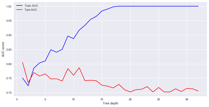
Let's first check for the best depth parameter for our decision tree.
- Create an array for for depth values ranging from 1 - 32.
- In a loop, train the classifier for each depth value (32 runs)
- Calculate the training and test AUC for each run
- Plot a graph to show under/over fitting and optimal value
- Interpret the results
# Identify the optimal tree depth for given data


# Your code here
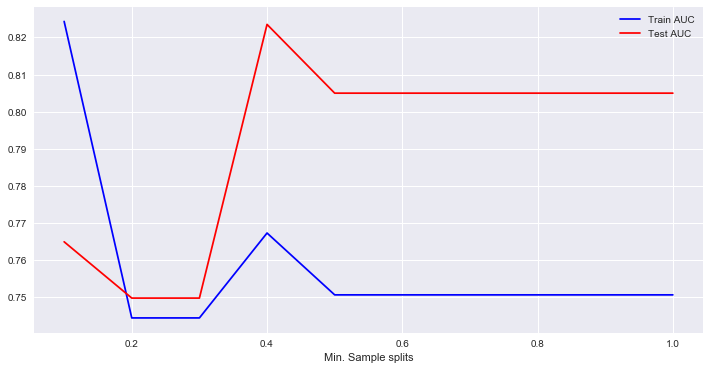
# You observations here Now check for the best min_samples_splits parameter for our decision tree.
- Create an array for for
min_sample_splitsvalues ranging from 0.1 - 1 with an increment of 0.1 - In a loop, train the classifier for each
min_samples_splitsvalue (10 runs) - Calculate the training and test AUC for each run
- Plot a graph to show under/over fitting and optimal value
- Interpret the results
# Identify the optimal min-samples-split for given data


# Your code here
# Your observations
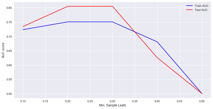
Now check for the best min_samples_leafs parameter value for our decision tree.
- Create an array for for
min_samples_leafsvalues ranging from 0.1 - 0.5 with an increment of 0.1 - In a loop, train the classifier for each
min_samples_leafsvalue (5 runs) - Calculate the training and test AUC for each run
- Plot a graph to show under/over fitting and optimal value
- Interpret the results
# Calculate the optimal value for minimum sample leafs

# Your code here
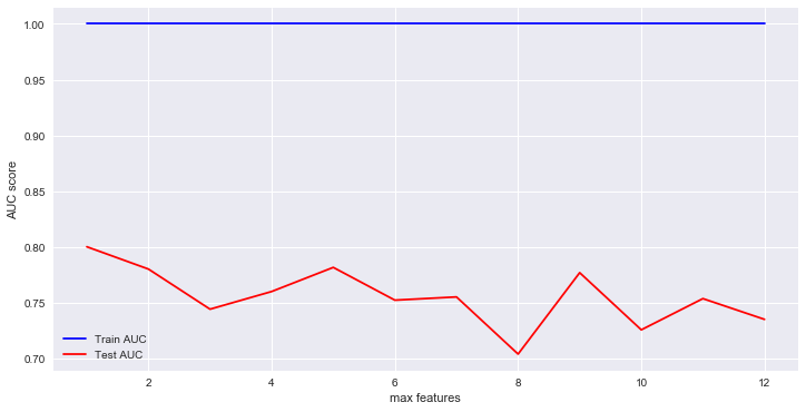
# Your observations here Now check for the best max_features parameter value for our decision tree.
- Create an array for for
max_featuresvalues ranging from 1 - 12 (1 features vs all) - In a loop, train the classifier for each
max_featuresvalue (12 runs) - Calculate the training and test AUC for each run
- Plot a graph to show under/over fitting and optimal value
- Interpret the results
# Find the best value for optimal maximum feature size


# Your code here
# Your observations here
So now we shall use the best values from each training phase above and feed it back to our classifier and see if have any improvement in predictive performance.
- Train the classifier with optimal values identified
- compare the AUC with vanilla DT AUC
- Interpret the results of comparison
# train a classifier with optimal values identified above

# Your code here
0.7348379629629629
# You observations here In the next section, we shall talk about hyper-parameter tuning using a technique called "grid-search" to make this process even more granular and decisive.
In this lesson, we looked at tuning a decision tree classifier in order to avoid over fitting and increasing the generalization capabilities of the classifier. For the Titanic dataset, we see that identifying optimal parameter values can result in some improvements towards predictions. This idea will be exploited further in upcoming lessons and labs.


