This project was assigned to me in Flatiron School's Immersive Data Science Program. The goal of the project is to analyze King County home sale data over a two year period (2015 and 2016) and find out how a residential real estate investor can gain a foothold in this market.
Housing prices in King County, WA have been exploding over the past decade due to many factors including the availability of great jobs, a rich culture, and an outdoor recreation opportunities in the surrounding areas. It is now harder than ever for house hunters to find a bargain in what seems like is a total sellers' market.
My goal in this project was to understand where, when, and what type of houses are available at decent prices and develop a multiple linear regression model capable of giving an indication whether or not investor should bargain. Meeting this goal required careful data cleaning, exploratory data analysis, thoughtful feature engineering, and finally an iterative approach to mutliple regression modelling.
Three questions explored:
- Question1: location
- Question2: timing
- Question3: other attributes which have impact on price.
In addition, Multiple Linear Regression analysys peformed to provide accurate predictions for house prices.
This project was created using the following languages and libraries. An environment with the correct versions of the following libraries will allow re-production and improvement on this project.
- Python version: 3.6.9
- Matplotlib version: 3.0.3
- Seaborn version: 0.9.0
- Pandas version: 0.24.2
- Numpy version: 1.16.2
- Statsmodels version: 0.9.0
- Scipy version: 1.2.1
- Sklearn version: 0.20.3
- Clone this repository.
- Dataset can be found in the file "kc_house_data.csv".
- Check requirements in Technologies section above and download libraries if necessary.
This question will explore which part of the King county is most expensive, how location can affect house prices and the correlation between house prices and location. If there is high correlation between house price and location data, location data can be used as a predictor for linear regression analysis.
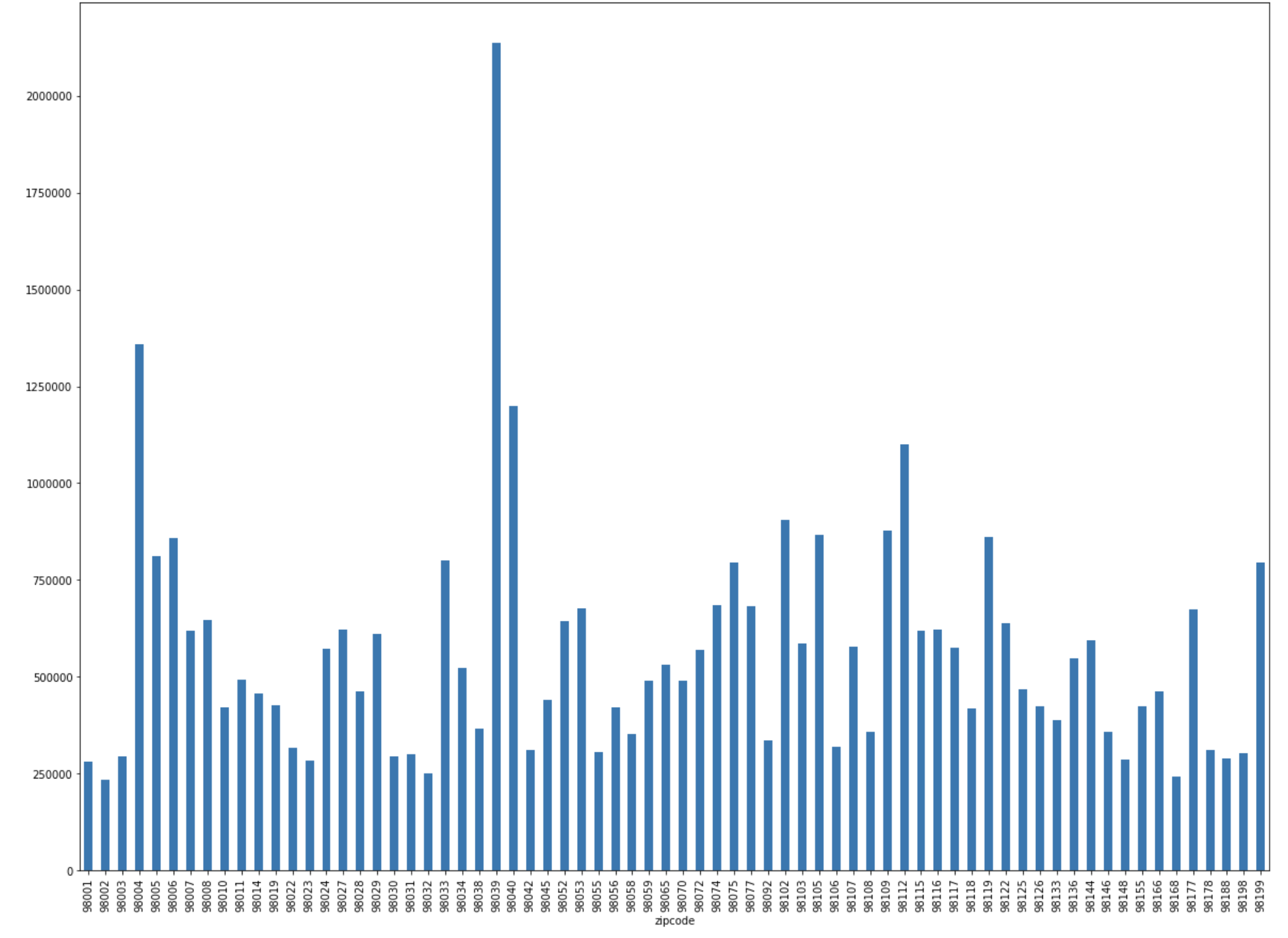
Average price calculated for each zip code and after grouping the prices by zip codes, the mean () function is used instead of sum () to reach better results.
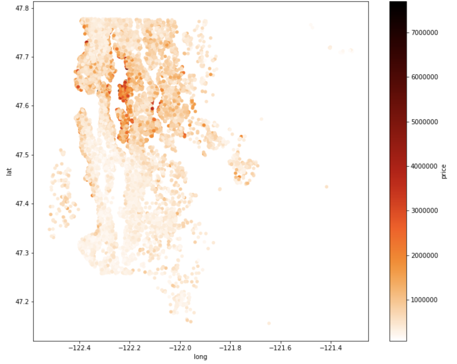
Direction column created to search how is average price distributed by directions. A scatter plot created with avaliable latitude and longitude data. To specify the four directions the scatter plot used as a base.
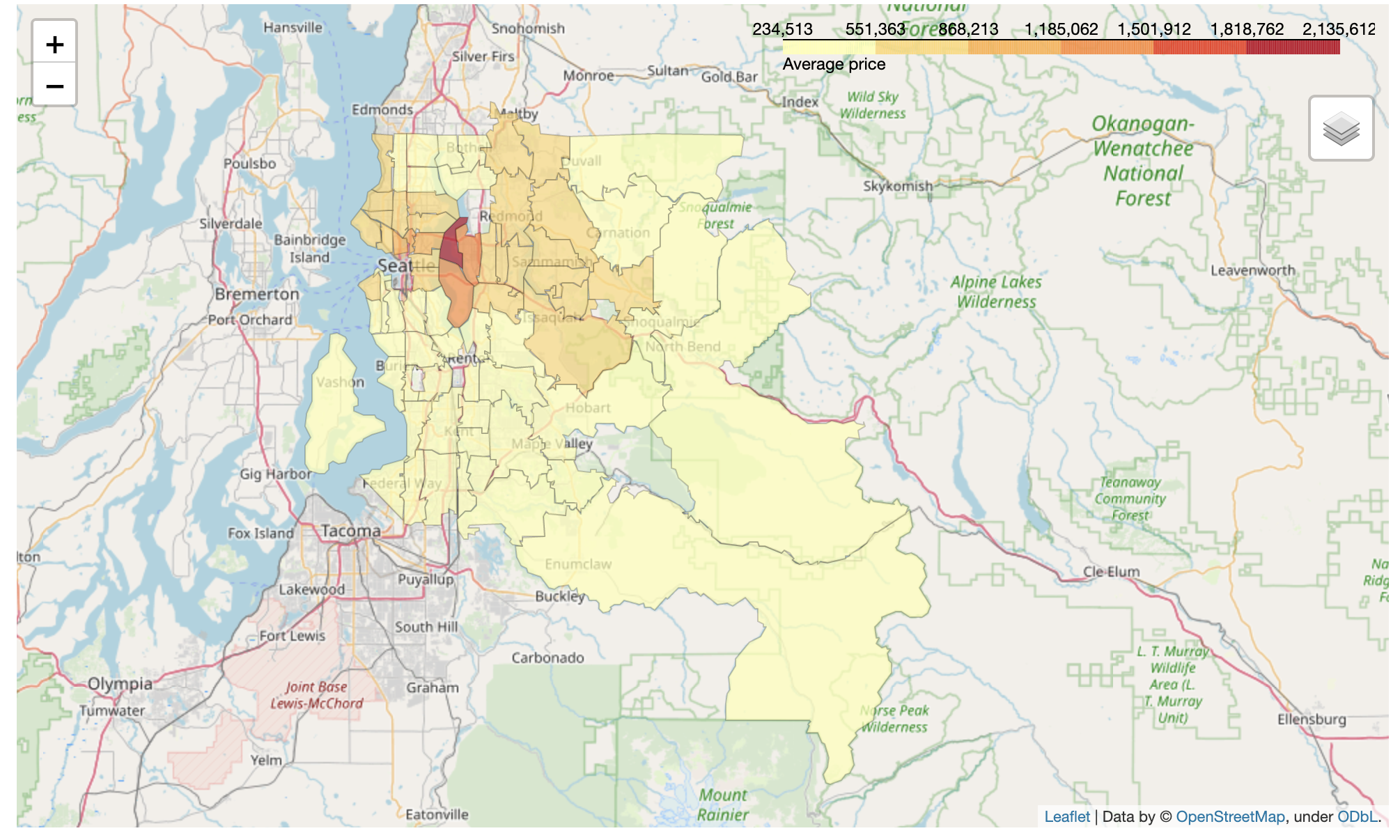
Four directions(NW, NE, SE, SE) calculated for each latitude and longitude combination and added to the dataframe. To analyze location's effect on house prices 'zipcode_king_county.geojson' is loaded to work with folium. It helped to create a heatmap with Choropleth() function showing average price for each zip code.
- The top 5 zip codes by average price are 98039, 98004, 98040, 98112 and 98102.
- Location is one of the most important features in predicting house prices.
- As expected the northwest of the county has the highest price and highest variance.
- It can be concluded that the Bellevue, Seattle and Mercer Island have the highest average house prices.
- Northeast is the second in terms of highest price and variance.
- Southwest and Southeast parts of the county has lowest prices.
- The average price for northeast and northwest are almost the same.
- The average price of southeast is higher than southwest part of the county.
- The results showed that location has hight impact on house prices therefore location data can be used as a proxy to predict house prices.
- More concrete insights can be reached with broader datasets including features such as crime rates, distance to transportation and schools etc.
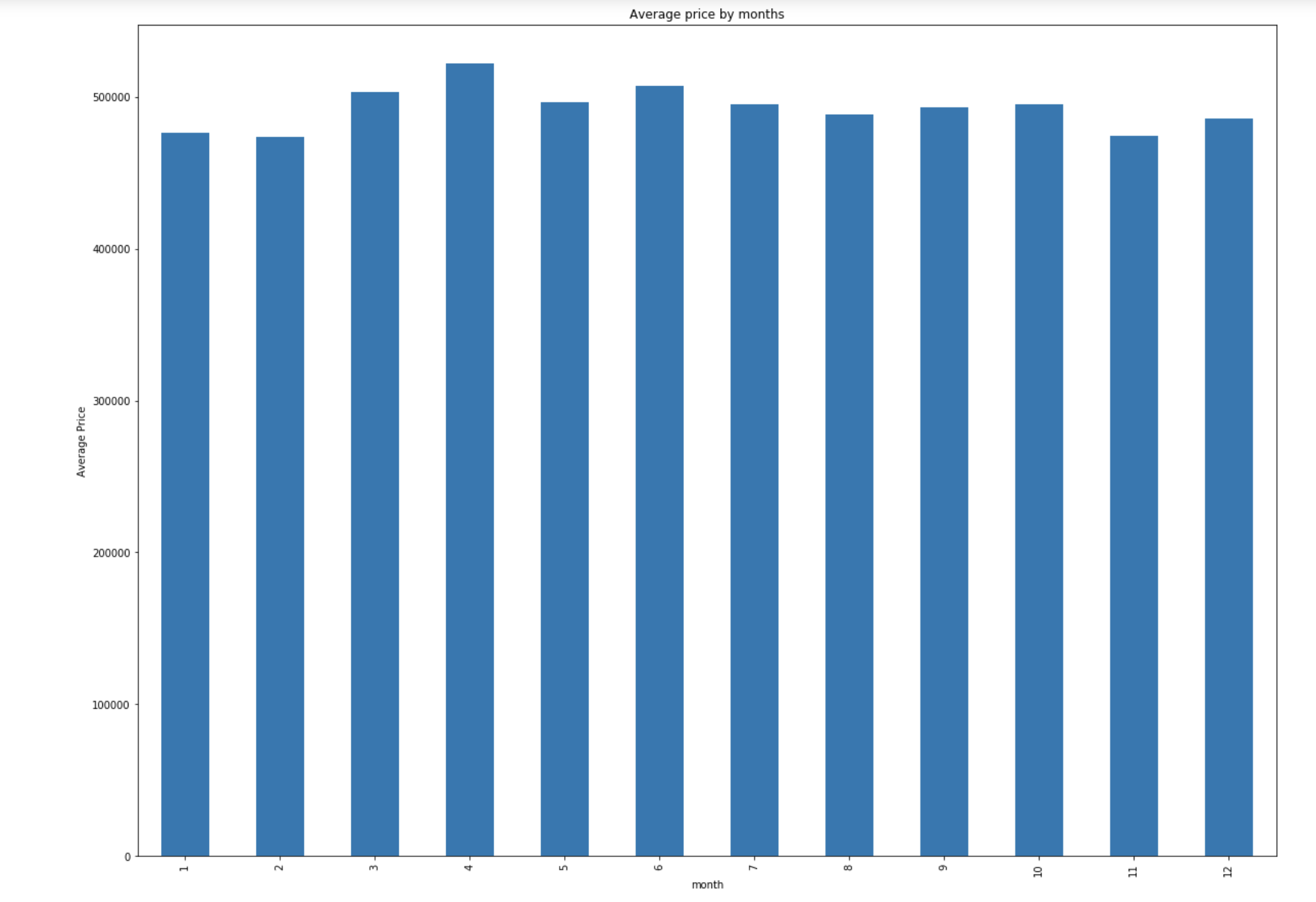
This question aims to answer which season and month is more affordable in terms of buying a house, as well as months and seasons role in predicting house prices. In order to answer our second question the 'month' and 'season' columns which are previously created and added to the dataframe are used. Furthermore, groupby() function is used to group data in months and seasons. During grouping the price by months and seasons, the mean () function is used to reach unbiased results.
- As predicted the best season to buy a house is winter.
- Fall has the highest price range followed by summer and spring.
- Spring has the highest average price followed by summer and fall.
- The average prices and median for each season are very close. Season is not genuine as expected to be used as a predictor in the regression model.
- While October has the highest variance, February has the lowest variance.
- February has the lowest, April has the highest price average.
- Like seasons there isn't a the big difference between the median values and average price for months.
- Month is also not an effective predictor for the regression model.
- The results showed that seaons and months has considerable low impact on house prices therefore season and month data cannot be used as an effective proxy to predict house prices.
- More concrete insights can be reached with broader datasets including a longer period of purchases.
Baseline model uses 'is_renovated', 'waterfront','with_basement', 'view', 'condition', 'condition_4', spring, summer,'spring','summer', grade, 'sqft_living','sqft_lot','sqft_above','sqft_living15','sqft_lot15','bathrooms' and 'yr_built' to predict the house prices. Some of them are added as dummy variables to the dataframe. The baseline model explains variance for 61 %.
For refining the model zip codes and directions are added to the second model as dummy variables. With the location feature the model's R-squared value reached to 87 %. To avoid multicollinearity 'sqft_above' value dropped and the R-squared value decreased by 0.001.
With Recursive Feature Elimination 70 features is chosen and the final model accounts for 85 % of the house prices.
The final model's mean squared values for test and train sets indicates that the final model is not ovetfitting or underfitting.


