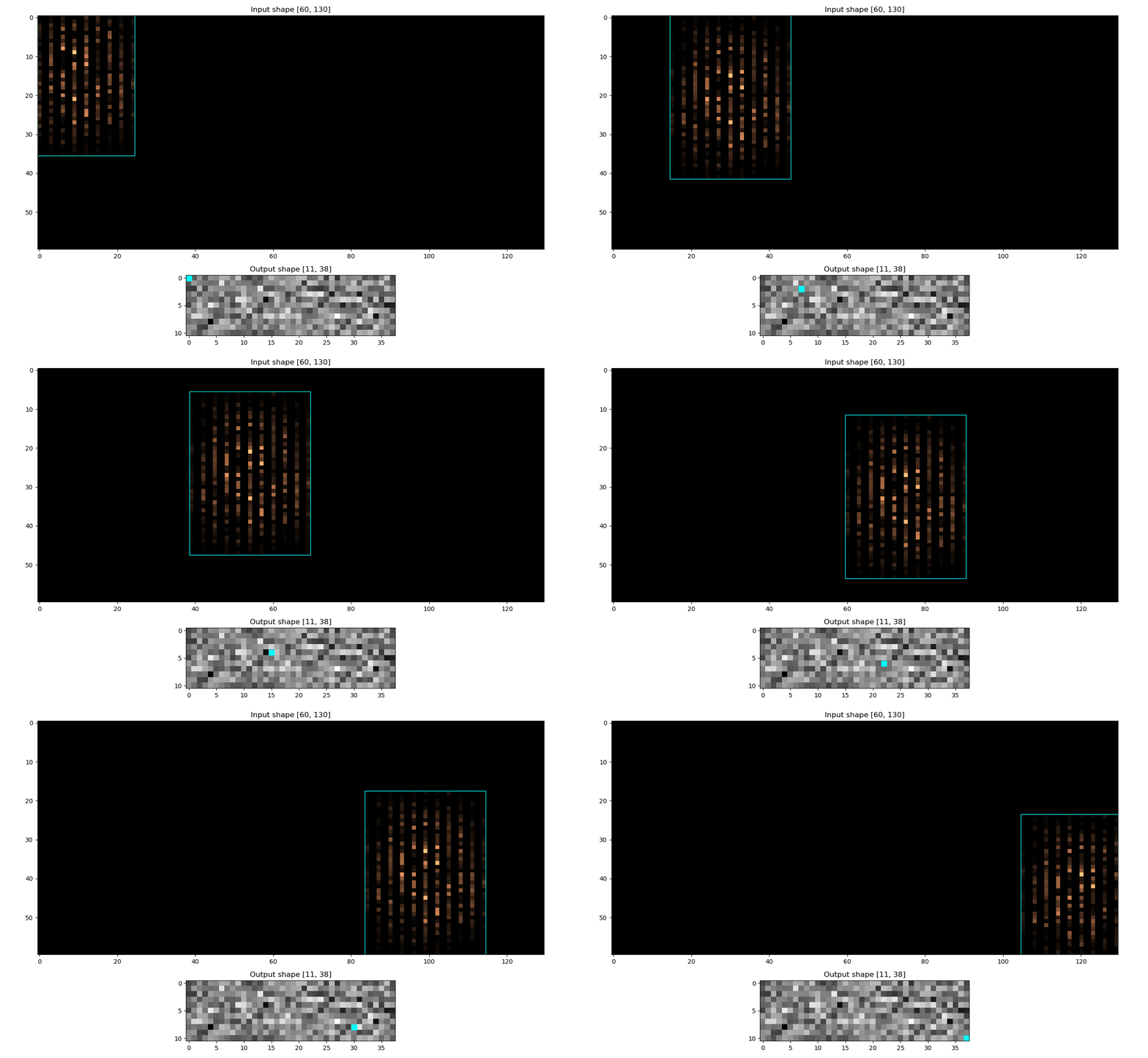
Analyzing the Receptive Field for a Convolutional Neural Network can be very useful in debugging and/or better understanding of how the model's output looked at the input.
The RF can be mathematically derived (a good blogpost on receptive field arithmetic and this excellent distill.pub). But we can also take advantage of automatic differentiation libraries to compute the RF numerically.
- Build the dynamic computational graph of the conv block
- Replace output gradients with all
0s - Pick a
(h, w)position in this new gradient tensor and set it tonon-zeros - Backprop this gradient through the graph
- Take the
.gradof the input after the backward pass, and look for non-zero entries
Can refer to the demo notebook or:
import torch
from numeric_rf import NumericRF

# ... given an image tensor `im`

convs = torch.nn.Sequential(
                                torch.nn.Conv2d(3, 16, (5,3), stride=(3,2)),
                                torch.nn.Conv2d(16, 16, (5,3), stride=2),
                                torch.nn.Conv2d(16, 16, 3, stride=2),
                                torch.nn.Conv2d(16, 16, 3, padding=1),
                                torch.nn.Conv2d(16, 8, 3),
        )

rf = NumericRF(model = convs, input_shape =  im.shape)

rf.heatmap(pos = (4, 8))

rf.info()

rf.plot(image = im, add_text = True)
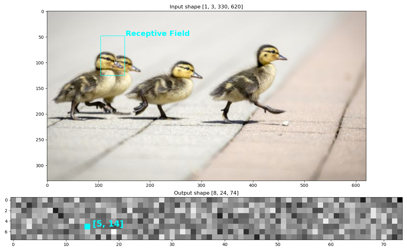
Will give both the receptive field for that output position:
{
	'h': {
		'bounds' : (18, 58),
		'range'  : 40},

	'w': {
		'bounds' : (28, 50),
		'range'  : 22}
}
And also the visualization:
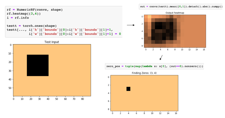
A quick way to verify that this approach works can be found in the demo notebook, by following these steps:
- Calculate the receptive field for the conv block at a given position (important to zero out the bias term!)
- Create an input shaped tensor of
1s - Zero out all input entries that fall in the Receptive Field
- After a forward pass, the only zero entry should be the chosen position (other factors may contribute to zeros in the output, e.g. padding, but the initial output position must be
0)
Illustrated here:


