NEWS v0.9 was a breaking release. See the news for details on how to update.
This package implements a variety of interpolation schemes for the Julia language. It has the goals of ease-of-use, broad algorithmic support, and exceptional performance.
Currently this package's support is best for B-splines and also supports irregular grids. However, the API has been designed with intent to support more options. Pull-requests are more than welcome! It should be noted that the API may continue to evolve over time.
Other interpolation packages for Julia include:
Some of these packages support methods that Interpolations does not,
so if you can't find what you need here, check one of them or submit a
pull request here.
At the bottom of this page, you can find a "performance shootout"
among these methods (as well as SciPy's RegularGridInterpolator).
Just
Pkg.add("Interpolations")
from the Julia REPL.
Note: the current version of Interpolations supports interpolation evaluation using index calls [], but this feature will be deprecated in future. We highly recommend function calls with () as follows.
Given an AbstractArray A, construct an "interpolation object" itp as
itp = interpolate(A, options...)where options... (discussed below) controls the type of
interpolation you want to perform. This syntax assumes that the
samples in A are equally-spaced.
To evaluate the interpolation at position (x, y, ...), simply do
v = itp(x, y, ...)Some interpolation objects support computation of the gradient, which can be obtained as
g = Interpolations.gradient(itp, x, y, ...)or as
Interpolations.gradient!(g, itp, x, y, ...)where g is a pre-allocated vector.
Some interpolation objects support computation of the hessian, which can be obtained as
h = Interpolations.hessian(itp, x, y, ...)or
Interpolations.hessian!(h, itp, x, y, ...)where h is a pre-allocated matrix.
A may have any element type that supports the operations of addition
and multiplication. Examples include scalars like Float64, Int,
and Rational, but also multi-valued types like RGB color vectors.
Positions (x, y, ...) are n-tuples of numbers. Typically these will
be real-valued (not necessarily integer-valued), but can also be of types
such as DualNumbers if
you want to verify the computed value of gradients.
(Alternatively, verify gradients using ForwardDiff.)
You can also use
Julia's iterator objects, e.g.,
function ongrid!(dest, itp)
    for I in CartesianIndices(itp)
        dest[I] = itp(I)
    end
end
would store the on-grid value at each grid point of itp in the output dest.
Finally, courtesy of Julia's indexing rules, you can also use
fine = itp(range(1,stop=10,length=1001), range(1,stop=15,length=201))There is also an abbreviated notion described below.
The interpolation type is described in terms of degree and, if necessary, boundary conditions. There are currently four degrees available: Constant, Linear, Quadratic, and Cubic corresponding to B-splines of degree 0, 1, 2, and 3 respectively.
B-splines of quadratic or higher degree require solving an equation system to obtain the interpolation coefficients, and for that you must specify a boundary condition that is applied to close the system. The following boundary conditions are implemented: Flat, Line (alternatively, Natural), Free, Periodic and Reflect; their mathematical implications are described in detail in the pdf document under /doc/latex.
When specifying these boundary conditions you also have to specify whether they apply at the edge grid point (OnGrid())
or beyond the edge point halfway to the next (fictitious) grid point (OnCell()).
Some examples:
# Nearest-neighbor interpolation
itp = interpolate(a, BSpline(Constant()))
v = itp(5.4)   # returns a[5]

# (Multi)linear interpolation
itp = interpolate(A, BSpline(Linear()))
v = itp(3.2, 4.1)  # returns 0.9*(0.8*A[3,4]+0.2*A[4,4]) + 0.1*(0.8*A[3,5]+0.2*A[4,5])

# Quadratic interpolation with reflecting boundary conditions
# Quadratic is the lowest order that has continuous gradient
itp = interpolate(A, BSpline(Quadratic(Reflect(OnCell()))))

# Linear interpolation in the first dimension, and no interpolation (just lookup) in the second
itp = interpolate(A, (BSpline(Linear()), NoInterp()))
v = itp(3.65, 5)  # returns  0.35*A[3,5] + 0.65*A[4,5]
There are more options available, for example:
# In-place interpolation
itp = interpolate!(A, BSpline(Quadratic(InPlace(OnCell()))))
which destroys the input A but also does not need to allocate as much memory.
BSplines assume your data is uniformly spaced on the grid 1:N, or its multidimensional equivalent. If you have data of the form [f(x) for x in A], you need to tell Interpolations about the grid A. If A is not uniformly spaced, you must use gridded interpolation described below. However, if A is a collection of ranges or linspaces, you can use scaled BSplines. This is more efficient because the gridded algorithm does not exploit the uniform spacing. Scaled BSplines can also be used with any spline degree available for BSplines, while gridded interpolation does not currently support quadratic or cubic splines.
Some examples,
A_x = 1.:2.:40.
A = [log(x) for x in A_x]
itp = interpolate(A, BSpline(Cubic(Line(OnGrid()))))
sitp = scale(itp, A_x)
sitp(3.) # exactly log(3.)
sitp(3.5) # approximately log(3.5)
For multidimensional uniformly spaced grids
A_x1 = 1:.1:10
A_x2 = 1:.5:20
f(x1, x2) = log(x1+x2)
A = [f(x1,x2) for x1 in A_x1, x2 in A_x2]
itp = interpolate(A, BSpline(Cubic(Line(OnGrid()))))
sitp = scale(itp, A_x1, A_x2)
sitp(5., 10.) # exactly log(5 + 10)
sitp(5.6, 7.1) # approximately log(5.6 + 7.1)These use a very similar syntax to BSplines, with the major exception
being that one does not get to choose the grid representation (they
are all OnGrid). As such one must specify a set of coordinate arrays
defining the knots of the array.
In 1D
A = rand(20)
A_x = collect(1.0:2.0:40.0)
knots = (A_x,)
itp = interpolate(knots, A, Gridded(Linear()))
itp(2.0)
The spacing between adjacent samples need not be constant, you can use the syntax
itp = interpolate(knots, A, options...)where knots = (xknots, yknots, ...) to specify the positions along
each axis at which the array A is sampled for arbitrary ("rectangular") samplings.
For example:
A = rand(8,20)
knots = ([x^2 for x = 1:8], [0.2y for y = 1:20])
itp = interpolate(knots, A, Gridded(Linear()))
itp(4,1.2)  # approximately A[2,6]
One may also mix modes, by specifying a mode vector in the form of an explicit tuple:
itp = interpolate(knots, A, (Gridded(Linear()),Gridded(Constant())))Presently there are only three modes for gridded:
Gridded(Linear())whereby a linear interpolation is applied between knots,
Gridded(Constant())whereby nearest neighbor interpolation is used on the applied axis,
NoInterpwhereby the coordinate of the selected input vector MUST be located on a grid point. Requests for off grid coordinates results in the throwing of an error.
missing data will naturally propagate through the interpolation,
where some values will become missing. To avoid that, one can
filter out the missing data points and use a gridded interpolation.
For example:
x = 1:6
A = [i == 3 ? missing : i for i in x]
xf = [xi for (xi,a) in zip(x, A) if !ismissing(a)]
Af = [a for a in A if !ismissing(a)]
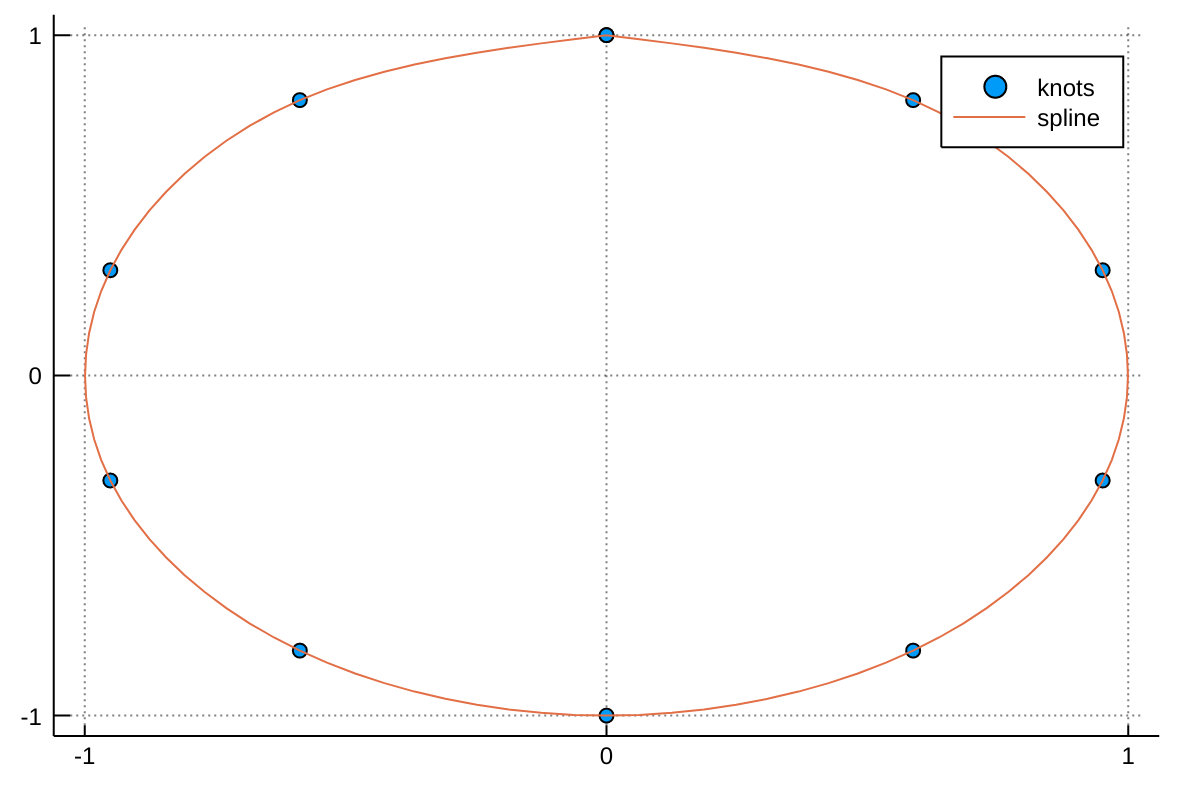
itp = interpolate((xf, ), Af, Gridded(Linear()))Given a set a knots with coordinates x(t) and y(t), a parametric spline S(t) = (x(t),y(t)) parametrized by t in [0,1] can be constructed with the following code adapted from a post by Tomas Lycken:
using Interpolations

t = 0:.1:1
x = sin.(2π*t)
y = cos.(2π*t)
A = hcat(x,y)

itp = scale(interpolate(A, (BSpline(Cubic(Natural(OnGrid()))), NoInterp())), t, 1:2)

tfine = 0:.01:1
xs, ys = [itp(t,1) for t in tfine], [itp(t,2) for t in tfine]
We can then plot the spline with:
using Plots

scatter(x, y, label="knots")
plot!(xs, ys, label="spline")The call to extrapolate defines what happens if you try to index into the interpolation object with coordinates outside of its
bounds in any dimension. The implemented boundary conditions are Throw, Flat, Linear, Periodic and Reflect,
or you can pass a constant to be used as a "fill" value returned for any out-of-bounds evaluation.
Periodic and Reflect require that there is a method of Base.mod that can handle the indices used.
Examples:
itp = interpolate(1:7, BSpline(Linear()))
etpf = extrapolate(itp, Flat())   # gives 1 on the left edge and 7 on the right edge
etp0 = extrapolate(itp, 0)        # gives 0 everywhere outside [1,7]
For linear and cubic spline interpolations, LinearInterpolation and CubicSplineInterpolation
can be used to create interpolating and extrapolating objects handily:
f(x) = log(x)
xs = 1:0.2:5
A = [f(x) for x in xs]

# linear interpolation
interp_linear = LinearInterpolation(xs, A)
interp_linear(3) # exactly log(3)
interp_linear(3.1) # approximately log(3.1)

# cubic spline interpolation
interp_cubic = CubicSplineInterpolation(xs, A)
interp_cubic(3) # exactly log(3)
interp_cubic(3.1) # approximately log(3.1)
which support multidimensional data as well:
f(x,y) = log(x+y)
xs = 1:0.2:5
ys = 2:0.1:5
A = [f(x,y) for x in xs, y in ys]

# linear interpolation
interp_linear = LinearInterpolation((xs, ys), A)
interp_linear(3, 2) # exactly log(3 + 2)
interp_linear(3.1, 2.1) # approximately log(3.1 + 2.1)

# cubic spline interpolation
interp_cubic = CubicSplineInterpolation((xs, ys), A)
interp_cubic(3, 2) # exactly log(3 + 2)
interp_cubic(3.1, 2.1) # approximately log(3.1 + 2.1)
For extrapolation, i.e., when interpolation objects are evaluated in coordinates outside the range provided in constructors, the default option for a boundary condition is Throw so that they will return an error.
Interested users can specify boundary conditions by providing an extra parameter for extrapolation_bc:
f(x) = log(x)
xs = 1:0.2:5
A = [f(x) for x in xs]

# extrapolation with linear boundary conditions
extrap = LinearInterpolation(xs, A, extrapolation_bc = Line())

@test extrap(1 - 0.2) # ≈ f(1) - (f(1.2) - f(1))
@test extrap(5 + 0.2) # ≈ f(5) + (f(5) - f(4.8))
You can also use a "fill" value, which gets returned whenever you ask for out-of-range values:
extrap = LinearInterpolation(xs, A, extrapolation_bc = NaN)
@test isnan(extrap(5.2))
Irregular grids are supported as well; note that presently only LinearInterpolation supports irregular grids.
xs = [x^2 for x = 1:0.2:5]
A = [f(x) for x in xs]

# linear interpolation
interp_linear = LinearInterpolation(xs, A)
interp_linear(1) # exactly log(1)
interp_linear(1.05) # approximately log(1.05)In the perf directory, you can find a script that tests
interpolation with several different packages. We consider
interpolation in 1, 2, 3, and 4 dimensions, with orders 0
(Constant), 1 (Linear), and 2 (Quadratic). Methods include
Interpolations BSpline (IBSpline) and Gridded (IGridded),
methods from the Grid.jl
package, methods from the
Dierckx.jl package, methods
from the
GridInterpolations.jl
package (GI), methods from the
ApproXD.jl package, and
methods from SciPy's RegularGridInterpolator accessed via PyCall
(Py). All methods
are tested using an Array with approximately 10^6 elements, and
the interpolation task is simply to visit each grid point.
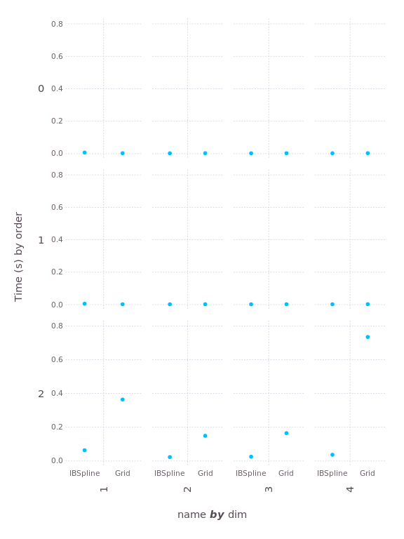
First, let's look at the two B-spline algorithms, IBspline and
Grid. Here's a plot of the "construction time," the amount of time
it takes to initialize an interpolation object (smaller is better):
The construction time is negligible until you get to second order (quadratic); that's because quadratic is the lowest order requiring the solution of tridiagonal systems upon construction. The solvers used by Interpolations are much faster than the approach taken in Grid.
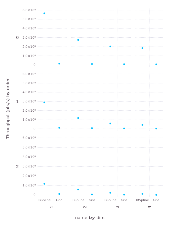
Now let's examine the interpolation performance. Here we'll measure "throughput", the number of interpolations performed per second (larger is better):
Once again, Interpolations wins on every test, by a factor that ranges from 7 to 13.
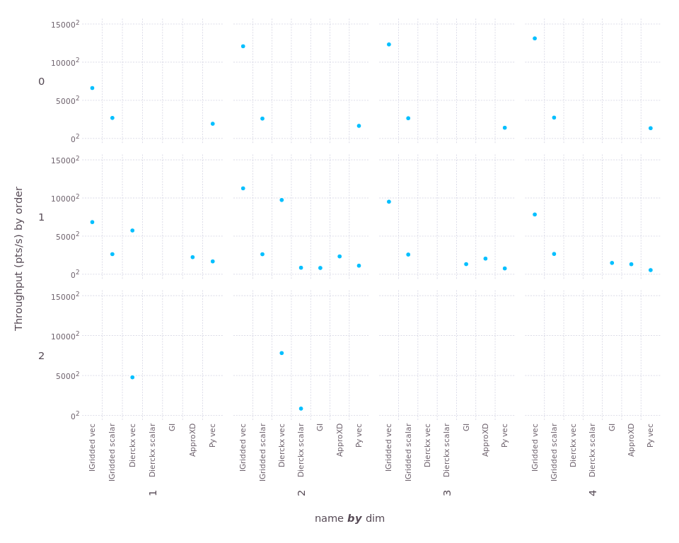
Now let's look at the "gridded" methods that allow irregular spacing
along each axis. For some of these, we compare interpolation performance in
both "vectorized" form itp[xvector, yvector] and in "scalar" form
for y in yvector, x in xvector; val = itp[x,y]; end.
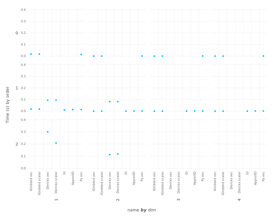
First, construction time (smaller is better):
Missing dots indicate cases that were not tested, or not supported by the package. (For construction, differences between "vec" and "scalar" are just noise, since no interpolation is performed during construction.) The only package that takes appreciable construction time is Dierckx.
And here's "throughput" (larger is better). To ensure we can see the wide range of scales, here we use "square-root" scaling of the y-axis:
For 1d, the "Dierckx scalar" and "GI" tests were interrupted because they ran more than 20 seconds (far longer than any other test). Both performed much better in 2d, interestingly. You can see that Interpolations wins in every case, sometimes by a very large margin.
Work is very much in progress, but and help is always welcome. If you want to help out but don't know where to start, take a look at issue #5 - our feature wishlist =) There is also some developer documentation that may help you understand how things work internally.
Contributions in any form are appreciated, but the best pull requests come with tests!
