This project is another tutorial for teaching you Artificial Neural Networks. I hope that my way of presenting the material will help you in the long learning process. All the examples are presented in TensorFlow and as a runtime environment
Project presents four different neural nets for MNIST digit classification. The former two are fully connected neural networks and latter are convolutional networks. Each network is built on top of the previous example with gradually increasing difficulty in order to learn more powerful models.
Project was implemented in Python 3 and Tensorflow v.1.0.0
- simple single layer neural network (one fully-connected layer),
- 5 layer Fully-connected neural network (5 FC NN) in 3 variants
- convolutional neural netowork: 3x convNet+1FC+output - activation function sigmoid
- convolutional neural netowork with dropout, relu, and better weight initialization: 3x convNet+1FC+output
This is the simplest architecture that we will consider. This feedforward neural network will be our baseline model for further more powerful solutions. We start with simple model in order to lay Tensorflow foundations:
- How to work with placeholders?
- What tensorflow varibales are?
- Understanding Tensorflow shapes and dimensions.
- Initalize TF session
- Run computations in a loop.
File: minist_1.0_single_layer_nn.py
This is simple one layer feedforward network with one input layer and one output layer
- Input layer 28*28= 784,
- Output 10 dim vector (10 digits, one-hot encoding)
input layer             - X[batch, 784]
Fully connected         - W[784,10] + b[10]
One-hot encoded labels  - Y[batch, 10]
Y = softmax(X*W+b)
Matrix mul: X*W - [batch,784]x[784,10] -> [batch,10]
Training consists of finding good W elements, this is handled automatically by Tensorflow Gradient Descent optimizer.
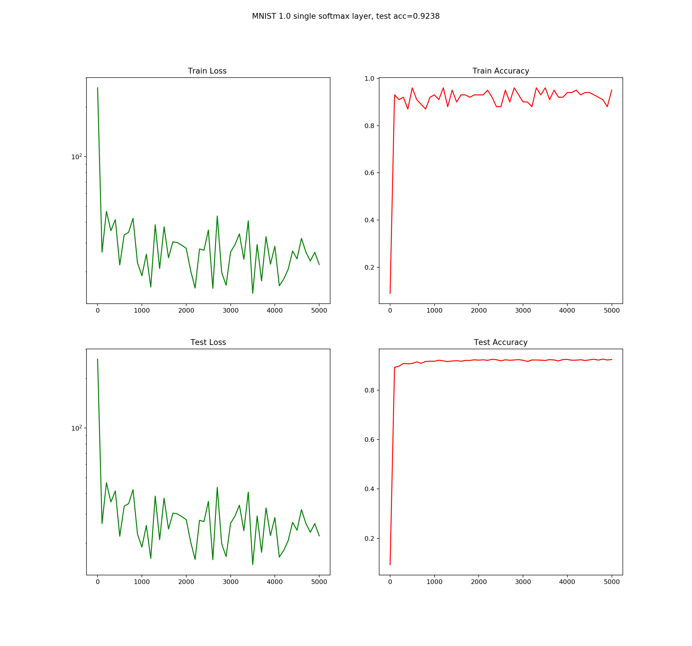
This simple model achieves 0.9237 accuracy
This is upgraded version of the previous model, between input and output we added five fully connected hidden layers. Adding more layers makes the network more expressive but in the same time harder to train. The three new problems could emerge vanishing gradients, model overfitting, and computation time complexity. In our case where the dataset is rather small, we did not see those problems in real scale.
In order to deal with those problems, different training techniques were invented. Changing from sigmoid to RELU activation function will prevent vanishing gradients, choosing Adam optimizer will speed up optimization and in the same time shorten training time, adding dropout will help with overfitting.
This model was implemented in three variants, where each successive variant builds on previous one and add some new features:
- Variant 1 is simple fully connected network with sigmoid activation function and Gradient descent optimizer
- Variant 2 use more powerful RELU activation function instead sigmoid and utilize better Adam optimizer
- Variant 2 add dropout usage in order to prevent overfitting
All variants share the same network architecture, all have five layers with sizes given below:
input layer             - X[batch, 784]
1 layer                 - W1[784, 200] + b1[200]
                          Y1[batch, 200]
2 layer                 - W2[200, 100] + b2[100]
                          Y2[batch, 200]
3 layer                 - W3[100, 60]  + b3[60]
                          Y3[batch, 200]
4 layer                 - W4[60, 30]   + b4[30]
                          Y4[batch, 30]
5 layer                 - W5[30, 10]   + b5[10]
One-hot encoded labels    Y5[batch, 10]

model
Y = softmax(X*W+b)
Matrix mul: X*W - [batch,784]x[784,10] -> [batch,10]
All results are for 5k iteration.
- five layer fully-connected : accuracy=0.9541
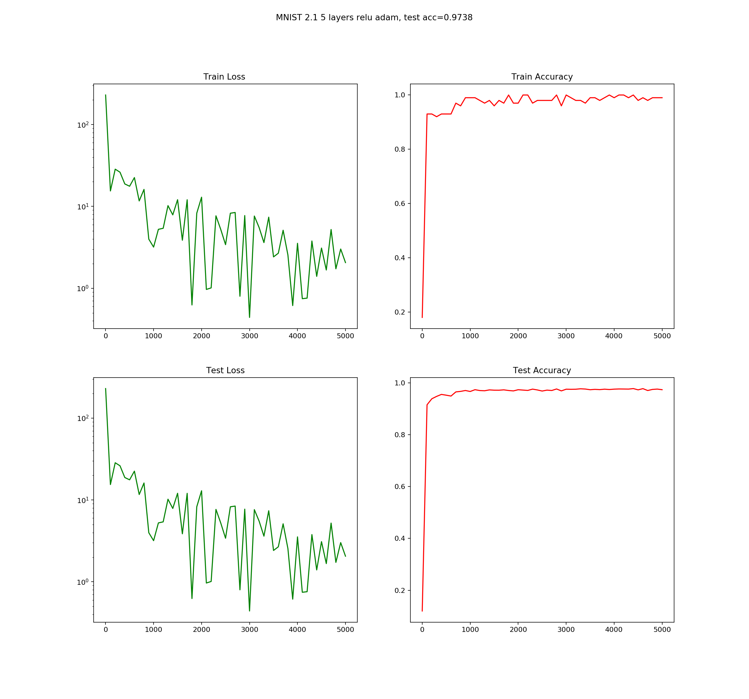
- five layer fully-connected with relu activation function and Adam optmizer: accuracy=0.9817
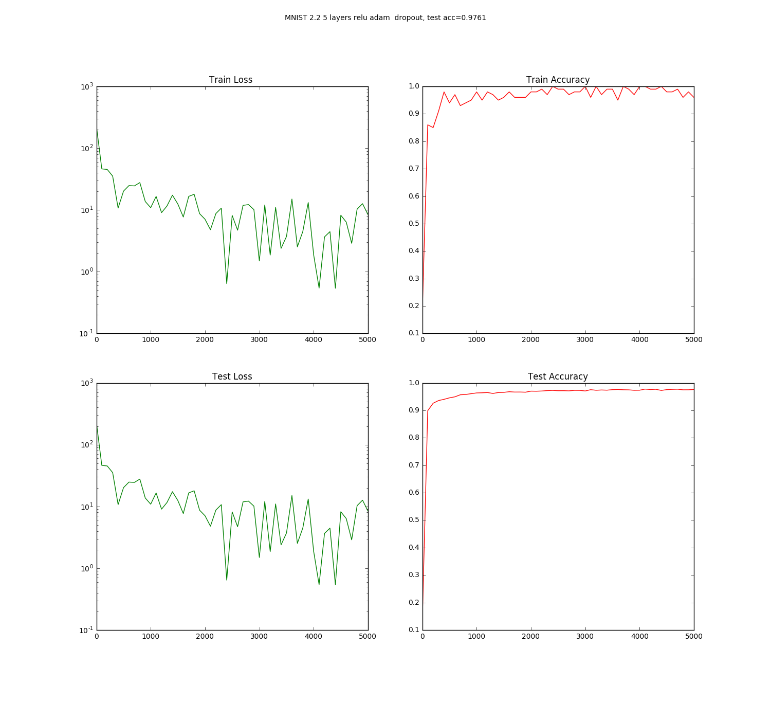
- five layer fully-connected with relu activation, Adam optmizer and dropout: accuracy=0.9761
As we can see changing from sigmoid to RELU activation and use Adam optimizer increase accuracy over 2.5%, which is significant for such small change. However, adding dropout decrease, but if we compare test loss graphs we can notice that dropout decrease the final test accuracy, but the test accuracy graph is much smoother.
The network layout is as follows:
5 layer neural network with 3 convolution layers, input layer 28*28= 784, output 10 (10 digits)
Output labels uses one-hot encoding
input layer               - X[batch, 784]
1 conv. layer             - W1[5,5,,1,C1] + b1[C1]
                            Y1[batch, 28, 28, C1]

2 conv. layer             - W2[3, 3, C1, C2] + b2[C2]
2.1 max pooling filter 2x2, stride 2 - down sample the input (rescale input by 2) 28x28-> 14x14
                            Y2[batch, 14,14,C2]
3 conv. layer             - W3[3, 3, C2, C3]  + b3[C3]
3.1 max pooling filter 2x2, stride 2 - down sample the input (rescale input by 2) 14x14-> 7x7
                            Y3[batch, 7, 7, C3]
4 fully connecteed layer  - W4[7*7*C3, FC4]   + b4[FC4]
                            Y4[batch, FC4]
5 output layer            - W5[FC4, 10]   + b5[10]
One-hot encoded labels      Y5[batch, 10]
As an optimizer I choose AdamOptimizer and all weights were randomly initialized from the Gaussian distribution with std=0.1. The activation function is RELU, without dropout.
All results are for 5k iteration.
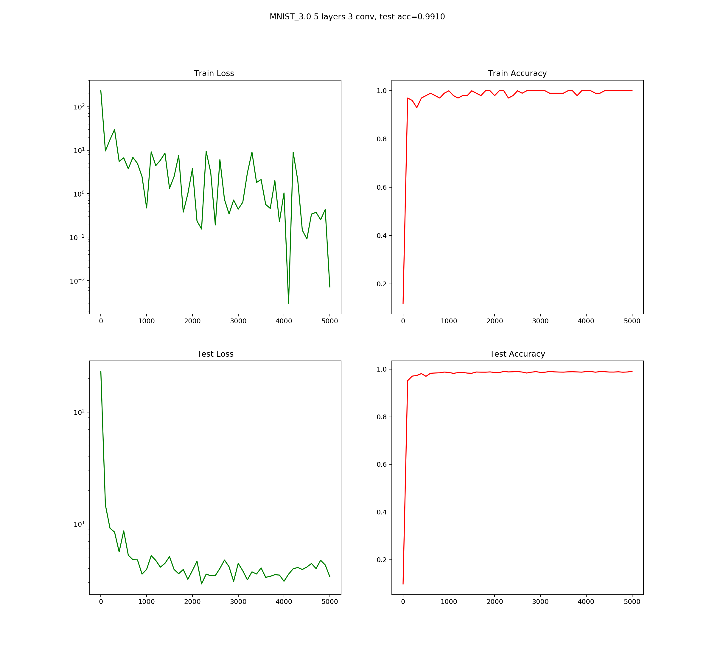
- five-layers convolutional neural network with max pooling: accuracy=0.9890
- Single layer neural network accuracy=0.9237
- five layer fully-connected : accuracy=0.9541
- five layer fully-connected with relu activation function and Adam optmizer: accuracy=0.9817
- five layer fully-connected with relu activation, Adam optmizer and dropout: accuracy=0.9761
- five layer convolutional neural network with max pooling : accuracy=0.9890
- CS231n Convolutional Neural Networks for Visual Recognition
- Tensorflow and deep learning without a Ph.D. - very good tutorial showing how to build modern MNIST conv net. It was my inspiration for this tutorial :)
- What is the difference between a Fully-Connected and Convolutional Neural Network?
- Tensorflow Examples by aymericdamien - GitHub repository with very useful and not so obvious Tensorflow examples
- Awesome tensorflow - A curated list of dedicated resources


