Information Processing Capacity

The information processing capacity (IPC) [1,2] is a measure to comprehensively examine computational capabilities of a dynamial system that receives random input ${\displaystyle u_t }#gh-light-mode-only$ ${\displaystyle\color{white} u_t }#gh-dark-mode-only$ . The system state ${\displaystyle x_t }#gh-light-mode-only$ ${\displaystyle\color{white} x_t }#gh-dark-mode-only$ holds the past processed inputs ${\displaystyle z_t }#gh-light-mode-only$ ${\displaystyle\color{white} z_t }#gh-dark-mode-only$ (e.g., ${\displaystyle z_t=u_{t-1},u_{t-2},u_{t-1}u_{t-2} }#gh-light-mode-only$ ${\displaystyle\color{white} z_t=u_{t-1},u_{t-2},u_{t-1}u_{t-2} }#gh-dark-mode-only$ ). We emulate the processed inputs ${ z_t }#gh-light-mode-only$ ${\color{white} z_t }#gh-dark-mode-only$ with linear regression of the state as follows:

Subsequently, we quantify the IPC as the amount of the held input using the following emulation accuracy:

${\displaystyle C = 1 - \frac{\sum_t (\hat{z}_t-z_t)^2}{\sum_t z_t^2}. }#gh-light-mode-only$

${\displaystyle\color{white} C = 1 - \frac{\sum_t (\hat{z}_t-z_t)^2}{\sum_t z_t^2}. }#gh-dark-mode-only$

Under the assumption that the state is a function of only input history ${\displaystyle x_t = f(u_{t-1},u_{t-2},\ldots) }#gh-light-mode-only$ ${\displaystyle\color{white} x_t = f(u_{t-1},u_{t-2},\ldots) }#gh-dark-mode-only$ , the total capacity ${\displaystyle C_{\rm tot} }#gh-light-mode-only$ ${\displaystyle\color{white} C_{\rm tot} }#gh-dark-mode-only$ , which is the summation of IPCs over all types of ${\displaystyle z_t }#gh-light-mode-only$ ${\displaystyle\color{white} z_t }#gh-dark-mode-only$ , is equivalent to the rank of correlation matrix ${\displaystyle r }#gh-light-mode-only$ ${\displaystyle\color{white} r }#gh-dark-mode-only$ (see [1,2] for further details).

Environment

The scripts use a GPU to compute IPCs fast and adopt CuPy library for multiprocessing.

Google Colaboratory

If you do not have available GPU(s), you can use Google Colaboratory, which provides a free GPU with 12 GB memory (as of Jun 7th, 2022). Here is the sample code of sample1_esn.ipynb on Google Colaboratory. Note that, if 12-hour time limit is over or it is not used for 90 minutes, it will shut down and erase your data.

Using your GPU

Please install required libraries through the following procedure.

Check your CUDA version by
```
/usr/local/cuda/bin/nvcc --version
```
Check your CuPy version here

Install the libraries by

pip install jupyter numpy matplotlib pandas cupy-cudaXXX

Example Codes

Echo state network

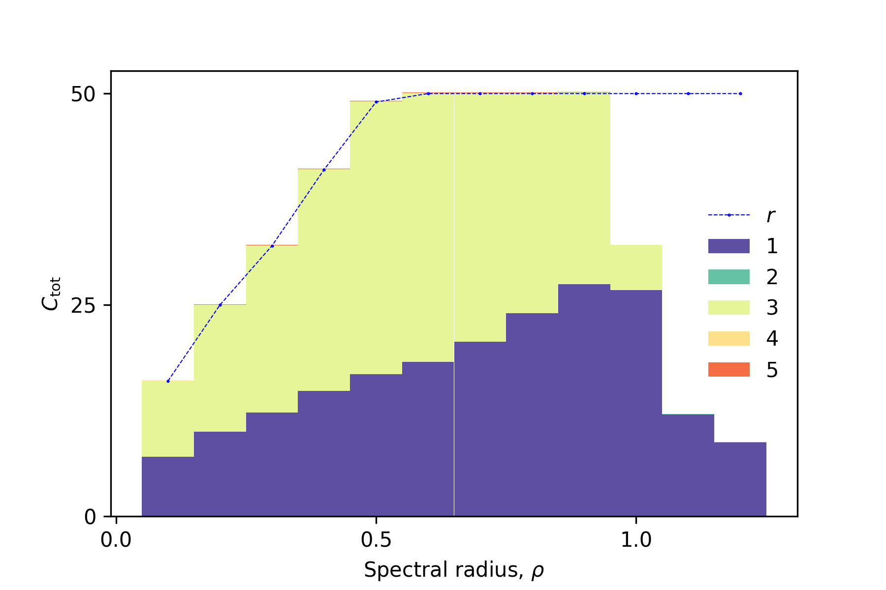
First, we demonstrate IPCs of an echo state network (ESN) to explain basic usage of the library. Please read sample1_esn.ipynb for details. After running it, we get the following IPC decomposion, which summarizes capacities for each order of input. The total capacity ${\displaystyle C_{\rm tot} }#gh-light-mode-only$ ${\displaystyle\color{white} C_{\rm tot} }#gh-dark-mode-only$ is equaivalent to the rank ${\displaystyle r }#gh-light-mode-only$ ${\displaystyle\color{white} r }#gh-dark-mode-only$ in the ordered region (the spectral radius ${\displaystyle \rho<1.0 }#gh-light-mode-only$ ${\displaystyle\color{white} \rho<1.0 }#gh-dark-mode-only$ ).
Memory functions

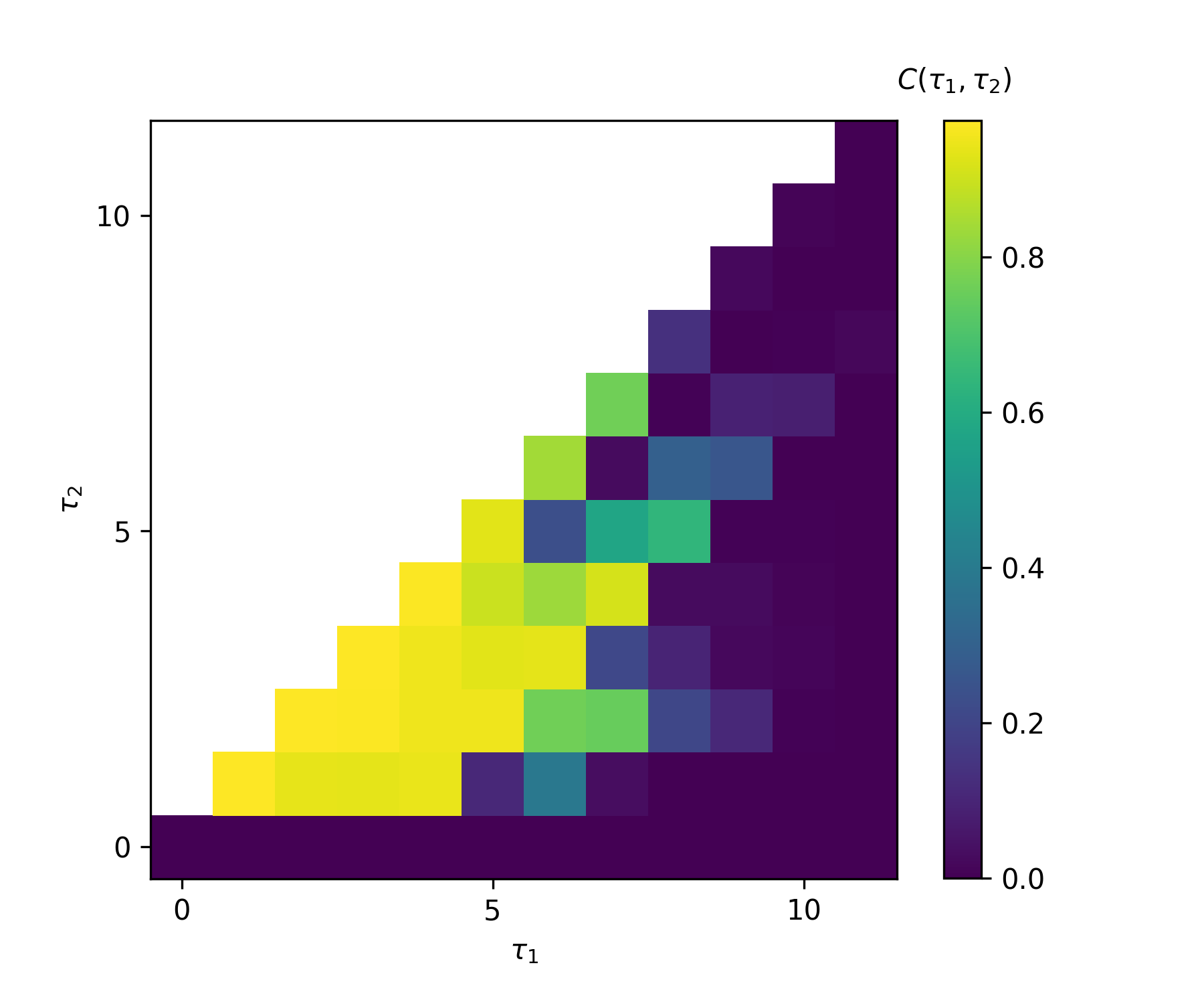
The IPC decomposition illustrates the degree of processed input but does not provide information on delays. To focus on memory length, sample2_memory_function.ipynb demonstrates how to depict first- and second-order memory functions.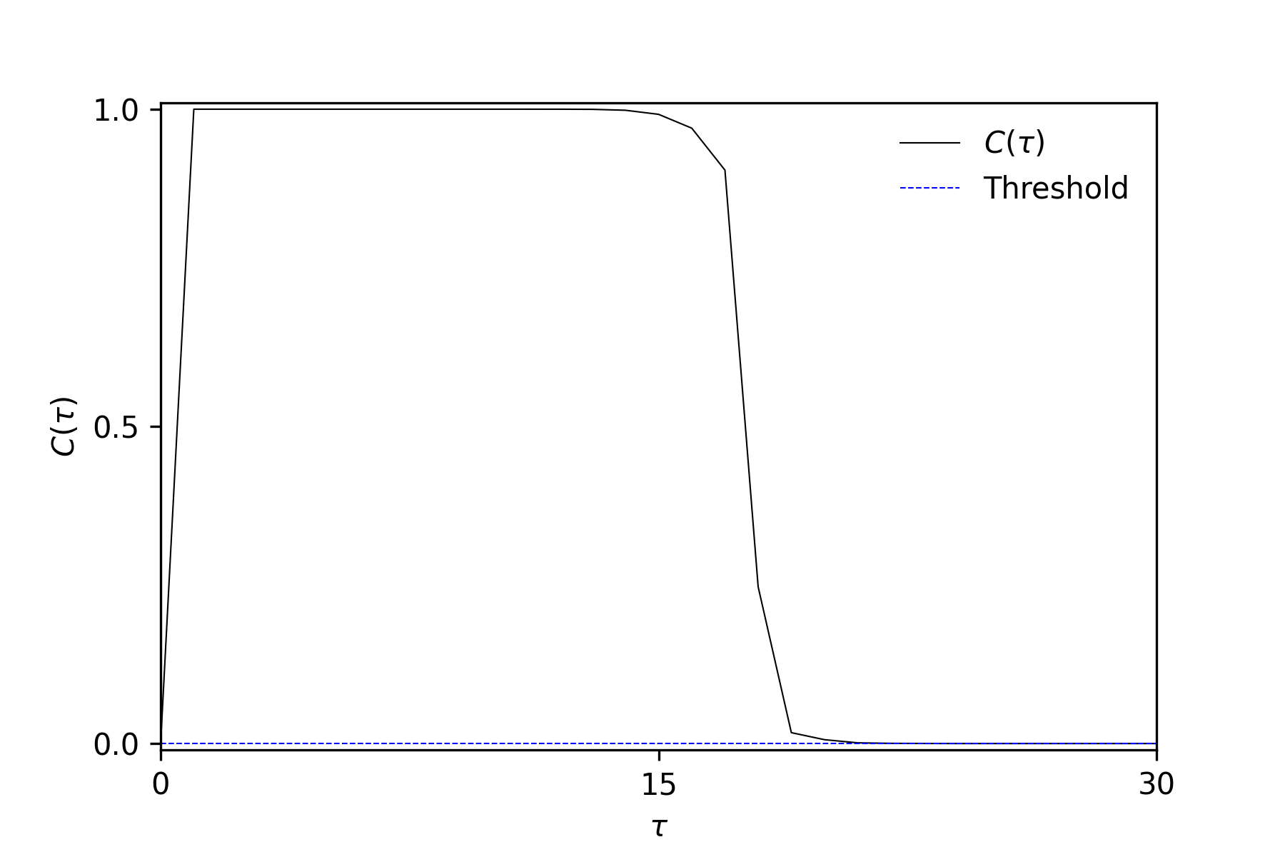

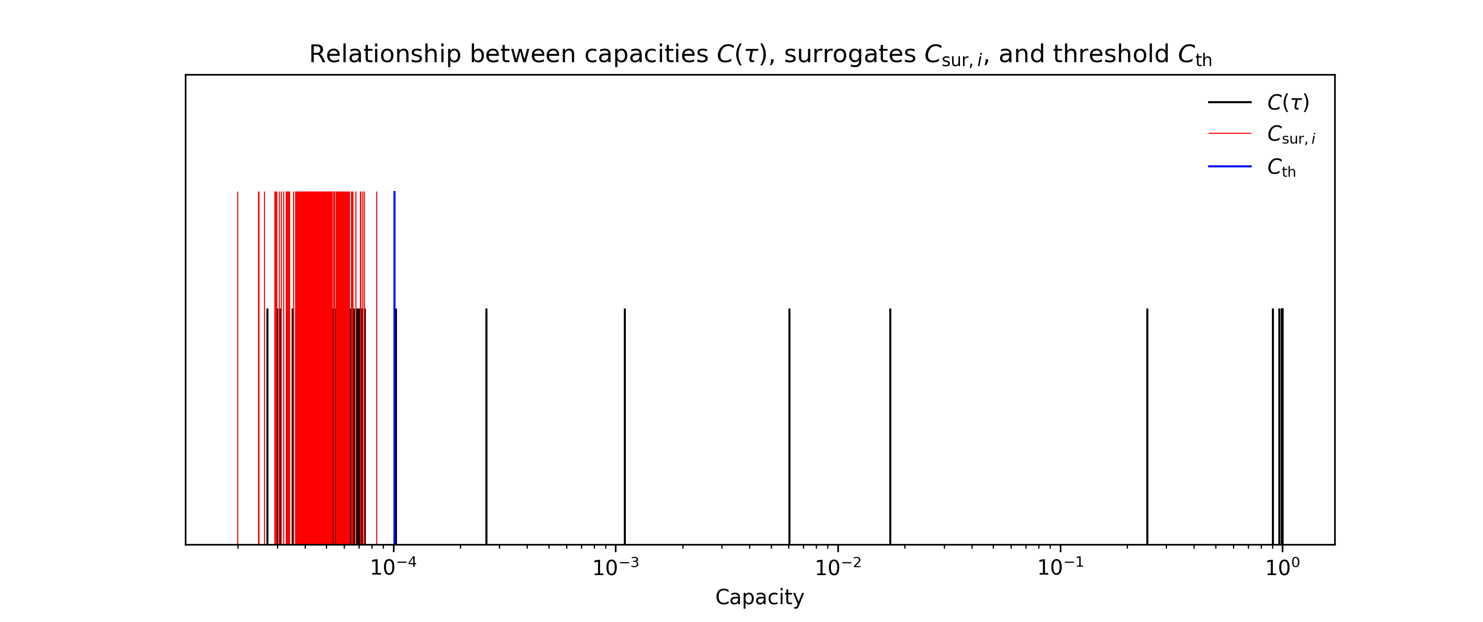
The capacities are calculated from time-series data with a finite length, which introduces a bias towards zero capacities. To eliminate the non-zero capacities, we use the shuffle surrogate method [2], which calculates a statistical threshold from surrogates. These surrogates are capacities calculated using target time-series that have been shuffled in the time direction, and they reflect the finite length of the time-series. If a capacity falls within the distribution of surrogates, we set its value to 0.
Individual IPC

When we would like to focus on not IPC summarized for each order but individual IPCs, we can easily compute and plot the individual ones. For example, the following figure illustrates the individual IPCs of the NARMA10 benchmark task model, ESN state, and output of NARMA10-trained ESN. sample3_individual.ipynb provides an example code to plot them.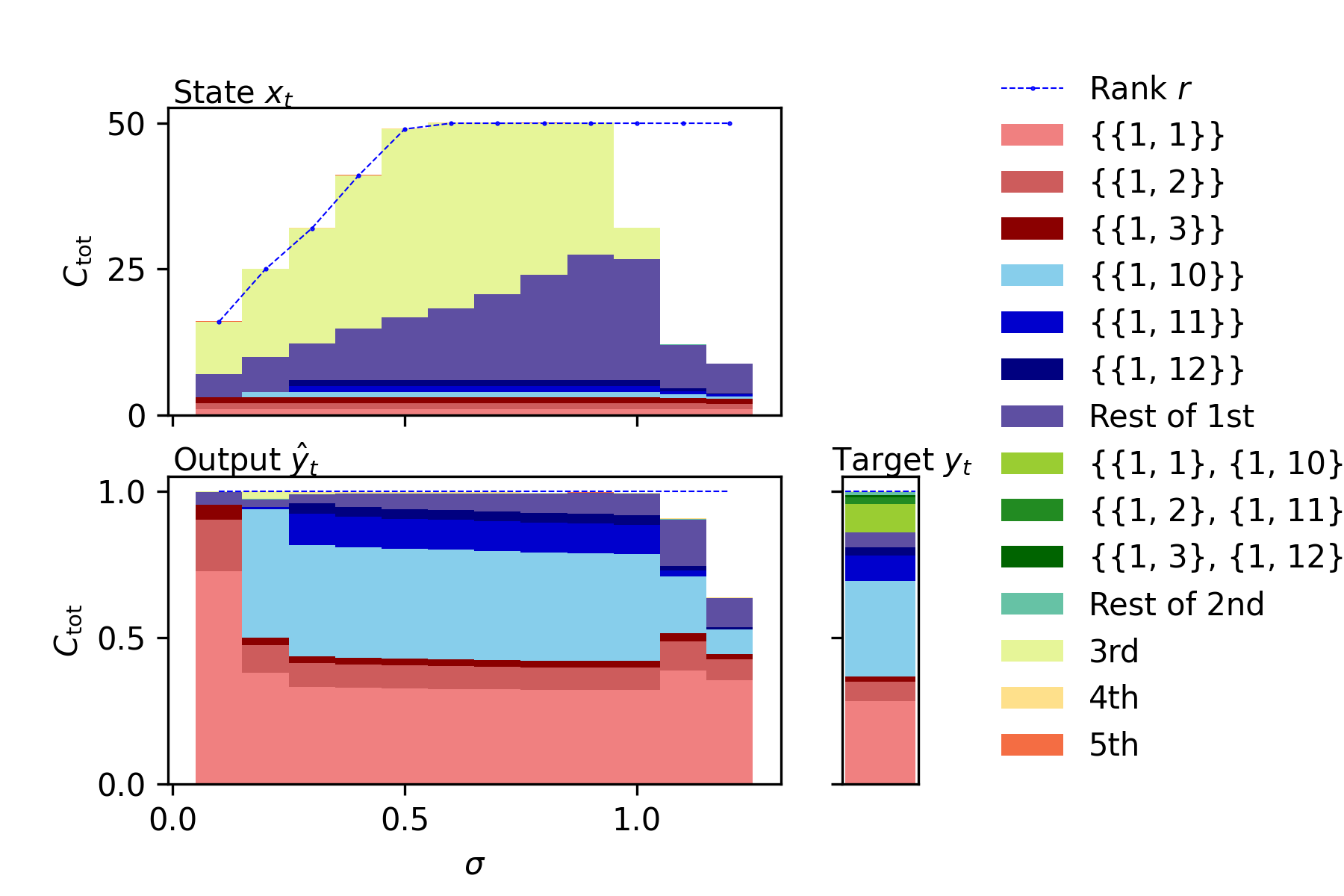
Input distribution

The input for IPC must be random but can follow an arbitrary type of distribution other than the uniform one [2]. sample4_dist.ipynb explains how to use seven other basic distributions. Even if your input distribution is not included in the eight ones, you can compute IPCs using arbitrary polynomial chaos (aPC) [2]. sample4_dist.ipynb also provides how to use aPC using a complex distribution such as a mixed Gaussian one.

If you compute IPCs of your reservoir, please replace input, state, and a set of degrees and delays with yours.

Release notes

version 0.10: A version for single input. You can compute IPCs using arbitrary input distribution except for bernoulli one.
version 0.11: We added sample3_individual.ipynb and information on Google Colaboratory. Also, we modified a bug in single_input_ipc.get_indivators().
version 0.12: ~~We modified bugs in ipc.singular_value_decomposition().~~ It turned out that they were not bugs, which occurred on Sep 23rd 2022 and were fixed on Jan 10th 2023 and might affect your system's rank and capacities. I deeply apologize for these mistakes.
version 0.13: We added sample2_memory_function.ipynb, as well as methods mf1d and mf2d.
version 0.14: We added explanations of the shuffle surrogate method to sample2_memory_function.ipynb.

References

[1] Joni Dambre, David Verstraeten, Benjamin Schrauwen, and Serge Massar. ''Information processing capacity of dynamical systems.'' Scientific reports 2.1 (2012): 1-7.

[2] Tomoyuki Kubota, Hirokazu Takahashi, and Kohei Nakajima. ''Unifying framework for information processing in stochastically driven dynamical systems.'' Physical Review Research 3.4 (2021): 043135.