Authors Kevin McDonough & Kyle Dufrane
Our stakeholder is a family that is moving to the Seattle area. They're looking for a solution that will enable them to search for properties.
This project uses the King County House Sales dataset, which can be found in KC_with_hoods.csv in the data folder in this repo. The description of the column names can be found in column_names.md in the same folder. Through our Linear Regression model we can show what elements have an effect on the sale price of a house and accurately predict what the price will be on similair properties. We found that the top two main factors on sale price are:
- Zip_city
- yr_renovated
This dataset contains house sale prices for King County, which includes Seattle. It includes homes sold between May 2014 and May 2015. In the datframe above, we used an API that allowed us to reverse geocode the latitude and longitude into neighborhoods. The code for this can be found in our individual technical notebooks. The process of reverse geocoding all 21,597 entries in our DataFrame took ~5 hours.
Our exploratory data analysis began with identifying feature types and null values. We eliminated all null values and replaced them with the median value of their respective columns due to the columns having a binary value. I.E. 1 in waterfront shows the house is waterfront while 0 shows the house is not waterfront property.
Next, we stripped the date column and created two separate columns (year and month). Once the columns were created we used the OrdinalEncoder to created new columns for each value within the column inturn this will add value to our model.
Once our data was cleaned, we identified our highest correlated columns to use in the model and dropped any that may negatively effect out model. When multicollinearity was identified (two columns correlating with eachother excluding the target (price)), we removed one of the values from the pair which had the least effect on the model. In total, we found two instances of two values having a high collinearity with each other. We chose to drop sqft_lot and sqft_above. See below results.
Lastly, we chose our relevant columns that would have a positive effect on the model. Please refer to techincal notebook for these columns.
Collinearity:
| Column | Collinearity |
|---|---|
| price | 1.000000 |
| prediction | 0.926310 |
| sqft_grade | 0.756248 |
| sqft_living | 0.701917 |
| grade | 0.667951 |
| sqft_living15 | 0.585241 |
| bathrooms | 0.525906 |
| view | 0.393497 |
| residual | 0.376762 |
| sqft_basement | 0.321108 |
| bedrooms | 0.308787 |
| waterfront | 0.264306 |
| floors | 0.256804 |
| sqft_lot15 | 0.082845 |
| yr_built | 0.053953 |
| condition | 0.036056 |
| Yr_sold | 0.003727 |
| zipcode | -0.053402 |
Multicollinearity:
| pairs | cc |
|---|---|
| sqft_above, sqft_living | 0.876448 |
| sqft_living, grade | 0.762779 |
| sqft_living15, sqft_living | 0.756402 |
| grade, sqft_above | 0.756073 |
| bathrooms, sqft_living | 0.755758 |
| sqft_living15, sqft_above | 0.731767 |
| sqft_lot15, sqft_lot | 0.718204 |
| grade, sqft_living15 | 0.713867 |
| price, sqft_living | 0.701917 |
| sqft_above, bathrooms | 0.686668 |
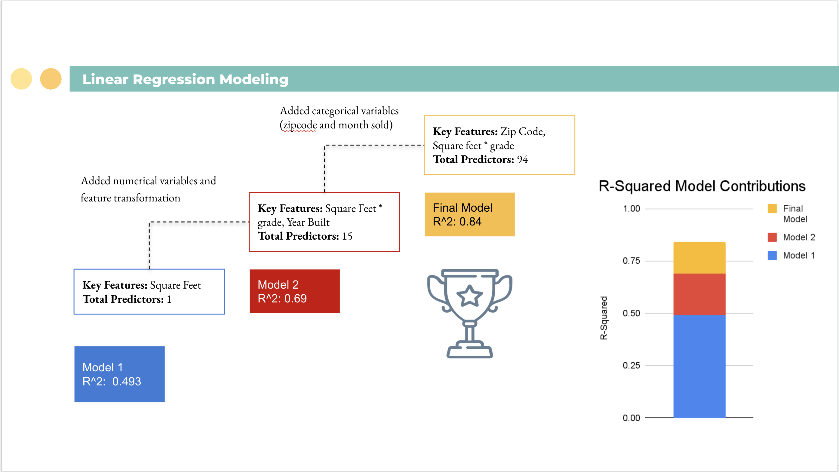
To take advantage of other correlations we used PolynomialFeatures from the sklearn.preprossing library. Our findings showed a strong correlation between square footage(x3) and grade(x9). Seeing this correlation we multiplied the columns by eachother and saw an increase in the R-squared value by 0.04.
PolynomnialFeatures(degree=2) results:
| col - val | Collinearity |
|---|---|
| x0 | 1.000000 |
| x0^2 | 0.839331 |
| x0 x1 | 0.937872 |
| x0 x2 | 0.917409 |
| x0 x3 | 0.900728 |
| x0 x5 | 0.908166 |
| x0 x8 | 0.945235 |
| x0 x9 | 0.982774 |
| x0 x10 | 0.890669 |
| x0 x12 | 0.999584 |
| x0 x13 | 0.938750 |
| x3 x9 | 0.756248 |
Lastly, for our final model, we used the OneHotEncoder through the sklearn.preprocessing library. We encoded three categorical values being the mo_sold (month sold), Zip_city (city & zip code), yr_renovated (year renovated).
Once these items were encoded our R-squared increased to 0.84.
Here is a brief overview of our model building process. For further detail please refer to the technical notebook.
Below are the Linear Regression assumption checks we used on our final model:
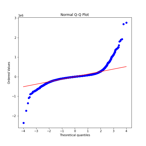
Q-Q Plot
There are tails on both sides of the q-q plot which, we believe, are due to location and square footage. We discuss this further in the technical notebook.
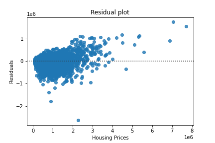
Heteroscedasticity
The heteroscedasticity are showing an identical story to the q-q plot. We have some outliers which our model under predicted the housing price which, we believe, is due to expensive neighborhoods having a higher price per square foot.
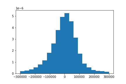
Normalization
This shows our normal distribution of our residuals.
Note: To utilize the interactive maps download a local web server(such as personal web server in the app store), download the files to your local pc, and open them in a local web browser OR go to the visualization folder and open within jupyter notebook.
Interactive Map based on a filter of 4 bedroom homes that are greater than 4750 sq ft
Interactive Map based on coefficients
Moving forward we want to identify what factors are causing the model to under or over predict. Also, we could plug in active houses on the market to direct our stakeholder to good under priced homes based on our model predictions.
Please review our full analysis in [our Jupyter Notebook](Technical Notebook.ipynb) or our presentation.
If you have any additional questions please contact either of us at:
Kyle Dufrane

    Email: kyle.dufrane@gmail.com
    Github: kyledufrane

 Kevin McDonough

     Email: kpmcdonough@gmail.com
     Github: KPMcDonough49
├── README.md
├── Technical_Notebook.ipynb
├── King_County_Presentation.pdf
├── data
└── Visualizations


