Forecasting 2.0 Accelerator
Forecasting 2.0 accelerator presentation
- Forecasting 2.0 Accelerator
- Overview
- I am a data scientist new to demand forecasting. How can this accelerator help me? What should I do to use it?
- Profiling (clustering) Time Series:
- Getting Started
- Functions
- Contributing
- Trademarks
Overview
This accelerator provides code and guidance to produce time series forecasting and time series profiling. The aim of this accelerator is to help data scientists to forecast multiple time series by building models based on the time-series profiling, by performing an accurate data preparation and by training and forecasting multiple time series based with models created ad-hoc for each profile.
Time series modelling is defined as the combination of:
- Choice of explanatory variables or regressors - which variables help me in explaining the target variable I want to forecast?
- Choice of forecasting algorithm - which algorithm do I use to produce my forecast? Arima, Linear regression, Boosting model?
- Choice of train set - how many observations do I use to train my model and produce my forecast?
Each model is optimized to better fit the training dataset and forecast the target variable: from energy consumption to spare parts demand. Classification or Clustering profile of time series data helps in defining the best fitting model in terms of choice of regressors (calendar variables or temperatures), forecasting algorithm (ARIMA vs Exponential smoothing) and train set (one year or just few days of data).
If I am new to demand forecasting, how can this accelerator help me? What should I do to use it?
What do I need in terms of time series data to use this accelerator?
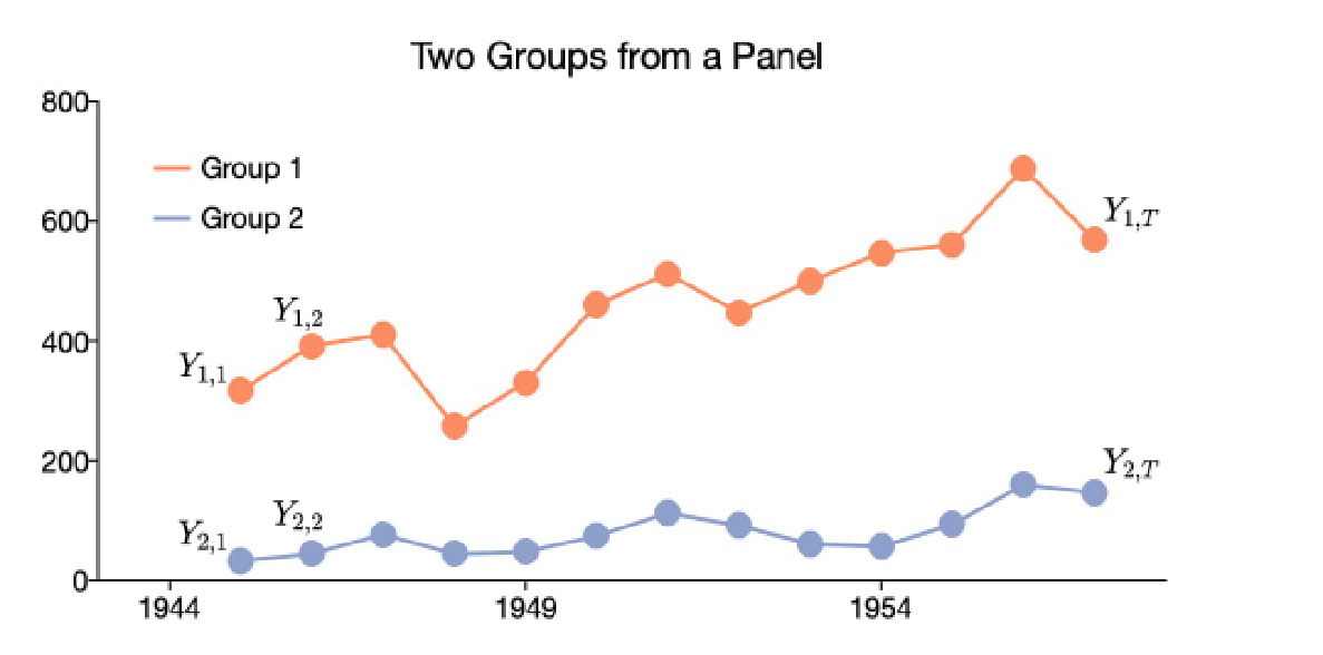
This accelerator deals with so-called panel data. In statistics and econometrics, panel data or longitudinal data is a collection of data that contains observations about different cross sections (groups or ids) that is assembled over intervals in time and ordered chronologically. Examples of groups that may make up panel data series include countries, firms, individuals, or demographic groups.
Specifically:
| Group or Id | Time period | Notation |
|---|---|---|
| 1 | 1 | |
| 1 | 2 | |
| 1 | T | |
| N | 1 | |
| N | 2 | |
| N | T |
Example datasets:
| Field | Topics | Example dataset |
|---|---|---|
| Microeconomics | GDP across multiple countries, Unemployment across different states, Income dynamic studies, international current account balances | Panel Study of Income Dynamics (PSID) |
| Macroeconomics | International trade tables, world socioeconomic tables, currency exchange rate tables | Penn World Tables |
| Epidemiology and Health Statistics | Public health insurance data, disease survival rate data, child development and well-being data | Medical Expenditure Panel Survey |
| Finance | Stock prices by firm, market volatilities by country or firm | Global Market Indices |
If you have a single time series it can be thought of as special cases of panel data that has one dimension only (one panel member or individual), so you can still take advantge from the accelerator, altought it is not useful to run the profiler, since you will have just one profile by default.
Why might this accelerator be useful for you
- It provides you with guidelines in the form of notebooks that can help you taking into account all necessary steps in order to perform a good data preparation, which is crucial in forecasting
- It provides you with a library of functions you might need when dealing with demand forecasting, such as:
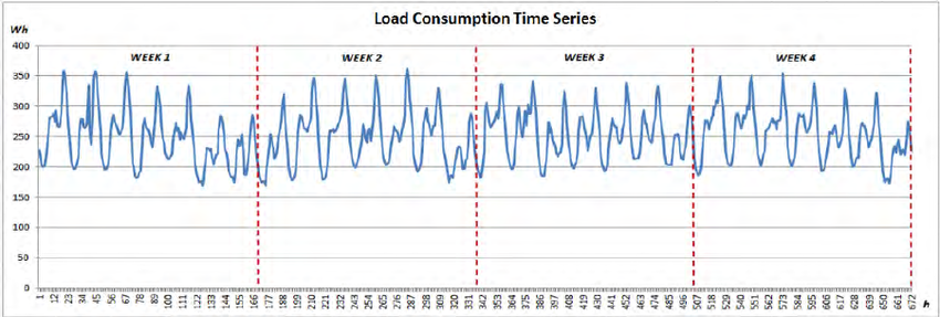
- Sliding plots like the one below:
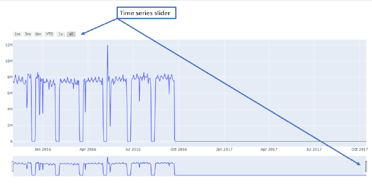
- Adding holidays by country or other regressors such as months, weekdays and interaction terms
- Creating normal temperature future scenarios to generate years-ahead forecasts
- Filling missing data using similar days or similar weeks values
- Compute errors like mean absolute error and mean absolute percentage error (also in case of zero dividend...)
- Wrap up results in Excel or csv files
- If you have several time series to forecast, thanks to the Profiling module, it allows you to quickly understand how "difficult" to forecast are the time series you are dealing with by classifying time series as intermittent or regular. You might want to know that if data profiling shows intermittent, you might not have consistent accuracy. This is crucial to drive the right customer expectations on the forecast accuracy. Profiling also helps you accelerating the production of forecast when dealing with high numbers of time series to forecast (more than 10 and less than 100): by grouping time series, for example with 2 intermittent + 4 regular consumption profiles, you can develop 6 models which can be applied by category thus reducing work load and increasing accuracy
- It helps you to quickly run backtesting with multiple models, and choosing the best model in terms of mean absolute error
How to use this accelerator as guideline
This accelerator provides you with 5 Notebooks that drives you through the essential steps you need to obtain a good forecast.
Notebooks
Notebooks are available in the Notebooks folder and provide guidance to use the Forecast 2.0 functions.
1. EnergyDataExploration
A notebook that provides an exploratory data analysis in order to understand the type of time series you are dealing with
2. EnergyPredictionDataPreparation
A notebook that helps with Time Series Data Preparation, in particular how to deal with NAs, how to aggregate time series and how to create useful regressors (e.g. calendar variables)
3. EnergyProfilingIntermittent
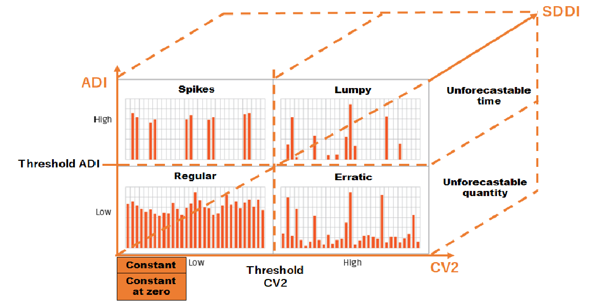
A notebook that profiles time series to be regular, intermittent, lumpy, erratic, unforecastable in terms of time, unforecastable in terms of quantity, constant and constant at zero
4. EnergyClusteringRegular
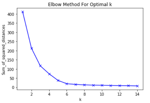
A notebook that performs a k-means flat cluster analysis on those time series that were classified as regular
5. EnergyPredictionScoring
A notebook that helps you produce a forecast, plot the results and compute KPIs on a panel dataframe, where you have multiple timeseries identified by a given group or id (e.g. multiple sensors time series, multiple plants or site-id energy consumption, etc)
How should I validate a model?
You can validate your model using the following KPIs (implemented, please refer to the EnergyPredictionScoring Notebooks and to the Functions section below):
Mean Error: average of all forecast-actualMean Absolute Error: average of all absolute values (forecast-actual)Mean Absolute Percentage Error: average of all absolute errors/actual
Interpreting errors
As you can infer, the above KPIs values depends on:
- Seasonality This means that when you have, for example, yearly seasonality, you might have periods of the year where the model performs better and where the model perform worse. Make sure which one is best for your use case.
- Low demand values This means that when you have, for example, a lot of low demand actual values and your forecast is in the neighbourhood of that value, your Absolute Percentage Error will easily result very close to 1, significantly worsening your MAPE. Make sure to interpret your error results accordingly.
Other important factors that can affect your error:
- Auto-regressive components If you have data that allows to employ auto-regressive components, i.e. the lagged value of the variable you want to forecast, this will improve your accuracy significantly.
- Length of forecast horizon If you need to forecast a long duration of horizon ahead (i.e. you start from daily data granularity and you need to forecast years ahead), your accuracy will reduce
- Measurement error If your data has a lot of outliers, missing data or measurement errors (i.e. sensors data), this will reduce your accuracy
- Collinearity Multicollinearity is a statistical concept where several independent variables in a model are correlated. Two variables are considered to be perfectly collinear if their correlation coefficient is +/- 1.0. Multicollinearity among independent variables will result in less reliable statistical inferences. You might consider using techniques such as Principal Component Analysis in order to deal with the issue.
Profiling (clustering) Time Series:
The goal is to identify consumption patterns that are similar to each other in order to assign the optimal model in terms of min of MAE or MSE.
The first step is to identify the series that is classified as “intermittent” with respect to those “regular” and then proceed to perform a k-means cluster analysis only on the latter.
The expected output is to label each time series as intermittent with respect to regular.
Identifying intermittent time series:
Definition of intermittent time series: intermittent time series or demand comes about when a product or a time series experiences several periods of zero demand. Often in these situation, when demand occurs it is small, and sometimes highly variable in size
How to identify intermittent time series:
Compute the following indicators such as
- Average Inter-demand Interval (ADI), this parameter is period based which is calculated as average interval time between two demand occurrences
- Coefficient of Variation Squared (CV2), this statistical parameter is calculated as standard deviation of the *For correspondence demand divided by the average demand for non-zero demand periods. The squared coefficient of variation represents variability of demand size.
- Standard Deviation of Inter-demand Interval (SDDI)
Based on their values, it is possible to identify intermittent time series as:
- spikes
- lumpy
- erratic
- unforecastable in terms of time volatility
- unforecastable in terms of quantity volatility
- constant
- constant at zero
- regular time series
Intermittent indicators parameters
Intermittent indicators parameters vary depending on the type of time series (i.e. data generation process of the time series) such as energy consumption in KWh or insurance claims in USD, therefore intermittent indicators must be set every time depending on the type of time series and their validation is done looking at time series charts resulting from the profiling Notebook.
Intermittent indicators are the following:
- thres_cv2_constant defines the threshold value to set constant time series with respect to a constant at zero time series
- thres_cv2 defines the threshold value between low CV2 and high CV2
- thres_adi defines the threshold value between low ADI and high ADI
- thres_sddi defines the threshold value between low SDDI and high SDDI
- min_time_cons defines the threshold value of minimum time between two demand entries (on with respect to off demand)
Parameters for electricity consumption in KWh, daily data.
- thres_cv2_constant = 0.06
- thres_cv2 = 2
- thres_adi = 3
- thres_sddi = 6.2
- min_time_cons = 2
Parameters for insurance claims data in USD, daily data. Claims from work accidents in mining industry.
- thres_cv2_constant = 0.01
- thres_cv2 = 0.2
- thres_adi = 1.2
- thres_sddi = 6.0
- min_time_cons = 25
What if I am working with data that are not related to energy consumption?
You can still use the accelerator and the profiler, but you need to setup new intermittent indicators. To do so, create a copy of the DataPreparation and ProfilingIntermittent Notebooks, run first the DataPreparation and save your data. Load them into the ProfilingIntermittent and having in mind the Intermittent Classificator Chart, set new parameters for thres_cv2_constant, thres_cv2, thres_adi, thres_sddi, min_time_cons and look if the resulting classification makes sense.
References on intermittent time series:
Methods to forecast intermittent time series (not yet implemented in this accelerator):
Constant
- Moving average
Constant at zero
- Moving average or actual zero value
Unforecastable time and unforecastable quantity
- Do not use a statistical model, it is better to develop a deterministic model (i.e. based on if/then rules)
Spikes, lumpy, erratic
- Croston’s method: Implementation in sktime
- Adjusted Croston methods
- Model-based forecasting methods
- ARMA models
- DARMA models -> Discrete ARMA
- INARMA models -> Integer-valued ARMA (INARMA)
Clustering profiles
- Clustering regular time series using K-Means flat
- Choose the optimal number of clusters
Methods to forecast regular time series
| # | Model | Library | Status | Notes |
|---|---|---|---|---|
| 1 | Linear regression | statsmodel | Implemented | |
| 2 | Gradient boosting | xgboost | Implemented | |
| 3 | Random forest | statsmodel | Implemented | |
| 4 | Kats | Kats | Not yet tmplemented | |
| 5 | Prophet | Prophet | Not yet implemented | Decompose into trend + season + holiday, etc |
| 6 | Neural networks | Neural prophet | Not yet implemented | |
| 7 | Probabilistic model | PyFlux | Not yet implemented | |
| 8 | Scikit-learn wrapper | Sktime | Not yet implemented | |
| 9 | Automatic time series | AutoTimeSeries | Not yet implemented | |
| 10 | Create synthetic time series for model testing | TimeSynth | Not yet implemented | |
| 11 | Computes series characteristics | Tsfresh | Not yet implemented | |
| 12 | ARIMA and deep NN | Darts | Not yet implemented | |
| 13 | Uber forecasting package | Orbit | Not yet implemented | pystan backend |
| 14 | Converting dates | Arrow | Not yet implemented | |
| 15 | Hydro(geo)logical time series analysis | Pastas | Not yet implemented | |
| 16 | Deep learning | Flow forecast | Not yet implemented | |
| 17 | Automating iterative tasks of machine learning model development | AutoML in Azure ML | Not yet implemented | |
| 18 | Netflix forecasting package | Metaflow | Not yet implemented |
Getting Started
-
Create a new conda environment named forecasting_energy using the
forecasting_energy_env.ymlin theEnvironmentfolder in the repository. To install a new environment using conda, you can access Anaconda navigator, click on import, name the new environment as forecasting_energy, select Python 3.8 and use the path to forecasting_energy_env.yml to install the new environment. Or you can use the following command:conda env create -f ./Environment/forecasting_energy.yml
-
To have an idea of software dependencies, read
requirements.txt -
Create a
config.yamlinConfigurationfolder, in order to run the code on your local machine/virtual machine. This is an example of the file(config.yaml)data_dir: input_path: "Data/Input" output_path: "Data/Output" plot_path: "Data/Plots"
-
Create your input, output and plot path
-
Load the test dataset from Kaggle, unzip and save it in your input folder
Default Directory Structure
├───Code     # Folder containing all the custom function created for this accelerator
│   ├───Plotting    # Plotting functions
│   └───Profiling   # Profiling time series functions
│       ├───Intermittent # Identification and classification of intermittent time series functions
│   └───Regressors # Create useful time series regressors, such as calendar variables or temperature transformations
│   └───Scoring # Create train and test sets, training, forecasting and computing KPIs functions
│   └───Utils   # Several utils functions called in the notebooks
├── Configuration # config.py that lead to config.yaml. with configuration
├───Docs # Additional documents
├───Notebooks     # Notebooks to do Profiling, Data Preparation, Scoring and Forecasting
├───Test     # Test Notebooks to do Profiling, Data Preparation, Scoring and Forecasting on various use cases
├── .gitignore
├── CODE_OF_CONDUCT.md
├── LICENSE.md
├── README.md
|── requirements.txt
├── SECURITY.md
└── SUPPORT.md
Build and Test
- Create a config.yaml as described above and compile it as:
- In data_dir set your folder tree for input, output and plot folder
- In saving choose your saving preferences
Functions
Functions are available in the Code folder.
Plotting
-
Class Plots
sliding_line_plot(df, serie_to_plot, id, i, chart_title="") -
Creates a sliding time series chart
sliding_fcst_plot(df, predict_col, expected_values, chart_title="", kpi=True)Creates a forecast vs actual sliding time series chart, with KPI option
Profiling
-
Class Intermittent
cv2_by_group(df, y, grouping_var, highest=0.05, lowest=0.05):
-
Computes cv2 by group
cv2(array, highest=0.05, lowest=0.05):
-
Winsorization is the process of replacing the extreme values of statistical data in order to limit the effect of the outliers on the calculations or the results obtained by using that data. The mean value calculated after such replacement of the extreme values is called winsorized mean.
adi(array, highest=0.05, lowest=0.05):
sddi(array, highest=0.05, lowest=0.05):
compute_indicator_values(vect, threshold, perc, quant, highest, lowest):
-
Computes indicator values
enh_compute_indicator_values(vect, threshold, perc, quant, highest, lowest):
Computes indicator values (enhanced)
Regressors
-
Class Regressors
create_interactions(df, var1, var2)
Adds interaction terms between two variables as var1*var2 to dataframe
create_non_linear_terms(df, var, n)
Adds non linear terms as var^2 to dataframe
add_holidays_by_country(df, date_var, country)
Adds holidays a dummy variable (0/1) to dataframe
add_weekdays(df, date_var)
Adds weekdays a dummy variables (0/1) for each weekday to dataframe
add_months(df, date_var)
Adds months a dummy variables (0/1) for each month to dataframe
calculate_degree_days(df, base_temperature, temperature)
Calculate the Degree Days Heating and Cooling values
merge_holidays_by_date(df, df_holidays, id)
Merge Holiday df with the train df
merge_additional_days_off(df, df_metadata, id, dict_days_off)
Merge Site Weekend data with train df
merge_weather(df, weather, date_var, id)
Merge weather data into the train df
-
Class SimilarDay:
get_similar_days_in_previous_year(dates, country)
Retrieves the similar day for a given date
get_similar_days_in_previous_week(dates, country)
Retrieves the similar day for a given date
get_similar_day_in_previous_year(d, holiday_calendar)
Retrieves the similar day for a given date. If the given date is not an holiday, the similar day is the closest day of the previous year in terms of calendar position which shares the weekday. If such a date is an holiday, the same weekday of the week before is considered.
get_similar_day_in_previous_week(d, holiday_calendar)
Retrieves the similar day for a given date. If the given date is not an holiday, the similar day is the closest day of the previous year in terms of calendar position which shares the weekday. If such a date is an holiday, the same weekday of the week before is considered. If the given date is an holiday, its similar day is the closest holiday to the given date in the previous year.
-
Class StandardConsumption:
get_standard_consumption_as_mean(df, id, date_var, var, country)
Retrieves the standard consumption for a given date as hourly monthly mean differentiated by holiday, weekend, weekdays
-
Class Temperatures:
ten_year(df, id, date_var = 'date_daily', start_date ='', end_date='31/12/2050')
Computes ten year averages temperatures and As-Is temperatures: where available use actual temp, if not use ten year averages
get_minimum_consumption(df, date_var, var, country)
Retrieves the minimum consumption for a given date as hourly monthly minimum value differentiated by holiday, weekend, night
Scoring
-
Class Training
train(dict_model_to_train, model)
Generate train
-
Class Forecasting
forecast(dict_test, trained_model)
Generate forecast
-
Class Scoring
find_best_algorithm(y, dict_train, dict_test, dict_algorithms, out_of_sample)
Finds the best performing algorithm in terms of min mean absolute error
stats_per_site(df, id, date_var)
Helper function to identify amount of data per site
resample_train_data(df, date_var, id, predict_col, sampling="D")Resample the data to a particular frequency
-
Class TrainTest
define_train_test_set_dates(df, y, train_start_date, train_end_date, test_start_date, test_end_date, test_size=0.33)
Defines train and test dates if left blank
def_train(df, y, list_id, train_start_date='', train_end_date='')
Define train dataset
def_test(df, y, list_id, test_start_date='', test_end_date='')
Define test dataset
Kpi
- Class Kpi
Compute mean absolute error
find_mae(y, dict_train, dict_test, dict_models):
Compute error as forecast-actualcompute_error(df, fcst, y):
Compute absolute error as abs(forecast-actual)compute_absolute_error(df, fcst, y):
Compute absolute % errorcompute_absolute_percentage_error(df, fcst, y):
Compute mean errorcompute_mean_error(df, fcst, y):
Compute mean absolute errorcompute_mae(df, fcst, y):
Compute mean absolute % errorcompute_mape(df, fcst, y):
Utils
-
Class Utils
def camel_to_snake(name)
Changes string from camel case to snake case
columns_camel_to_snake(df)
Changes dataframe columns from camel case to snake case
find_date(df)
Finds date columns in a dataframe
find_match_in_list(list_to_match, match_to_find):
Finds a match in a list given a list of possible words to match
delta_format(delta: np.timedelta64) -> str:Identifies frequency in numpy timedelta
find_freq(timedelta):
Finds frequency in numpy timedelta
find_freq_in_dataframe(df, date_var)
Finds frequency in pandas dataframe
create_folder_tree(folder_name)
creates folder tree
get_project_root(Path):
Finds the parent folder of the project
add_daily_date(df):
Adds a date variable at daily frequency to dataframe
find_categorical_variables(df):
Finds categorical variables in pandas dataframe
resample_data(df, id, date_var, sampling, dict_grouping)
Resample by aggregating the data to a particular frequency as defined in dict_grouping as {variable_to_resample: 'function_to_apply'}, i.e.{value: 'sum'}
resample_data(df, id, date_var, sampling, dict_grouping)
Resample by aggregating the data to a particular frequency (x-m,x-h,x-D) as defined (e.g. 3-M) in aggregation_per_col as{variable_to_resample: 'function_to_apply'}, i.e.{value: 'sum'}
add_seq(df, date_var, serie, freq, end_date='', start_date='')
Creates a sequence of complete date/hours to a dataframe
check_length_time_serie(df, date_var, index)
Checks the length that a time series of complete date/hours should have, so that it can be compared with actual observation
match_to_find(serie_to_find)
Finds a match in a list of possible words to match
find_match(df, serie_name, match_to_find):
Finds a match in a dataframe series given a list of possible words to match
find_match_in_list(list_to_match, match_to_find)
Finds a match in a list given a list of possible words to match
id_outliers_IQR(df, q1, q3, date_var, id, var, freq_var)
Identifies outliers creatinga dummy variable (0/1) called outlier using IQR method, where quantile value can be set
-
Class AlphabeticalCombinations
write_neat_csv(saving_file, df_fcst)
Writes neat csv
convert(string)
Convert string to list
excel_columns()Counts excel columns
write_beautiful_excel(saving_file, dict_df_to_write)
Writes beautiful excel
write_beautiful_excel_table(saving_file, dict_df_to_write)
Writes beautiful excel tables
Contributing
This project welcomes contributions and suggestions. Most contributions require you to agree to a Contributor License Agreement (CLA) declaring that you have the right to, and actually do, grant us the rights to use your contribution. For details, visit https://cla.opensource.microsoft.com.
When you submit a pull request, a CLA bot will automatically determine whether you need to provide a CLA and decorate the PR appropriately (e.g., status check, comment). Simply follow the instructions provided by the bot. You will only need to do this once across all repos using our CLA.
This project has adopted the Microsoft Open Source Code of Conduct. For more information see the Code of Conduct FAQ or contact opencode@microsoft.com with any additional questions or comments.
As data scientist, how can I contribute?
You can contribute both in extending the Profiling tool and in the data preparation and scoring part of this accelerator.
How to contribute to profiling?
What needs to be done is to test and define intermittent indicators (thres_cv2_constant, thres_cv2, thres_adi, thres_sddi, min_time_cons) for other types of data than electricity consumption, as reported below.
Insurance Claims data
Insurance claims data in USD, daily data. Claims from work accidents in mining industry.
- thres_cv2_constant = 0.01
- thres_cv2 = 0.2
- thres_adi = 1.2
- thres_sddi = 6.0
- min_time_cons = 25
How to contribute to data preparation and scoring?
What needs to be done is to improve the code to make it scalable and more efficient when working with big datasets (e.g. more than 100 id).
Trademarks
This project may contain trademarks or logos for projects, products, or services. Authorized use of Microsoft trademarks or logos is subject to and must follow Microsoft's Trademark & Brand Guidelines. Use of Microsoft trademarks or logos in modified versions of this project must not cause confusion or imply Microsoft sponsorship. Any use of third-party trademarks or logos are subject to those third-party's policies.

