This repository is forked from https://github.com/hoxo-m/densratio_py to change the outputs of the function. Instead of returning strings of detailed results and parameters, this module only returns the estimated values of The alpha-relative PE-divergence and KL-divergence between p(x) and q(x)
Density ratio estimation is described as follows: for given two data
samples x1 and x2 from unknown distributions p(x) and q(x)
respectively, estimate w(x) = p(x) / q(x), where x1 and x2 are
d-dimensional real numbers.
The estimated density ratio function w(x) can be used in many
applications such as the inlier-based outlier detection [1] and
covariate shift adaptation [2]. Other useful applications for density
ratio estimation were summarized by Sugiyama et al. (2012) in [3].
The package densratio provides a function densratio() that returns
an object with a method to estimate density ratio as
compute_density_ratio().
Further, the alpha-relative density ratio p(x)/(alpha * p(x) + (1 - alpha) * q(x)) (where alpha is in the range [0, 1]) can also be
estimated. When alpha is 0, this reduces to the ordinary density ratio
w(x). The alpha-relative PE-divergence and KL-divergence between
p(x) and q(x) are also computed.
For example,
import numpy as np
from scipy.stats import norm
from densratio import densratio

np.random.seed(1)
x = norm.rvs(size=500, loc=0, scale=1./8)
y = norm.rvs(size=500, loc=0, scale=1./2)
alpha = 0.1
densratio_obj = densratio(x, y, alpha=alpha)
print(densratio_obj)
gives the following output:
#> densratio_obj
#> (0.6536158708555955, 0.6214285743087546)
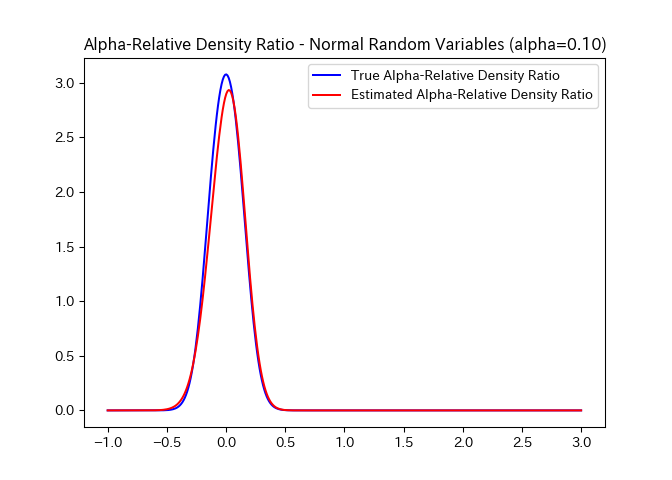
In this case, the true density ratio w(x) is known, so we can compare
w(x) with the estimated density ratio w-hat(x). The code below gives
the plot shown above.
from matplotlib import pyplot as plt
from numpy import linspace

def true_alpha_density_ratio(sample):
    return norm.pdf(sample, 0, 1./8) / (alpha * norm.pdf(sample, 0, 1./8) + (1 - alpha) * norm.pdf(sample, 0, 1./2))

def estimated_alpha_density_ratio(sample):
    return densratio_obj.compute_density_ratio(sample)

sample_points = np.linspace(-1, 3, 400)
plt.plot(sample_points, true_alpha_density_ratio(sample_points), 'b-', label='True Alpha-Relative Density Ratio')
plt.plot(sample_points, estimated_alpha_density_ratio(sample_points), 'r-', label='Estimated Alpha-Relative Density Ratio')
plt.title("Alpha-Relative Density Ratio - Normal Random Variables (alpha={:03.2f})".format(alpha))
plt.legend()
plt.show()You can install the package from PyPI.
$ pip install rulsif
Also, you can install the package from GitHub.
$ pip install git+https://github.com/kyosek/Relative-unconstrained-Least-Squares-Fitting.git
The source code for densratio package is available on GitHub at https://github.com/hoxo-m/densratio_py.
The package provides densratio(). The function returns an object that
has a function to compute estimated density ratio.
For data samples x and y,
from scipy.stats import norm
from densratio import densratio

x = norm.rvs(size = 200, loc = 1, scale = 1./8)
y = norm.rvs(size = 200, loc = 1, scale = 1./2)
result = densratio(x, y)
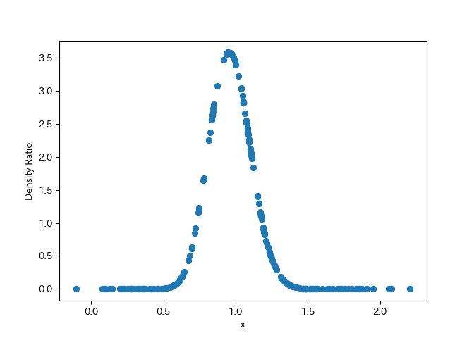
In this case, result.compute_density_ratio() can compute estimated
density ratio.
from matplotlib import pyplot as plt

density_ratio = result.compute_density_ratio(y)

plt.plot(y, density_ratio, "o")
plt.xlabel("x")
plt.ylabel("Density Ratio")
plt.show()The package estimates density ratio by the RuLSIF method.
RuLSIF (Relative unconstrained Least-Squares Importance Fitting) estimates the alpha-relative density ratio by minimizing the squared loss between the true and estimated alpha-relative ratios. You can find more information in Hido et al. (2011) [1] and Liu et al (2013) [4].
The method assumes that the alpha-relative density ratio is represented by a linear kernel model:
w(x) = theta1 * K(x, c1) + theta2 * K(x, c2) + ... + thetab * K(x, cb)
where K(x, c) = exp(- ||x - c||^2 / (2 * sigma ^ 2)) is the Gaussian
RBF kernel.
densratio() performs the following: - Decides kernel parameter sigma
by cross-validation. - Optimizes for kernel weights theta. - Computes
the alpha-relative PE-divergence and KL-divergence from the learned
alpha-relative ratio.
As the result, you can obtain compute_density_ratio(), which will
compute the alpha-relative density ratio at the passed coordinates.
densratio() outputs the result like as follows:
#> densratio_obj
#> (0.6536158708555955, 0.6214285743087546)
- First value is an estimated relative PE Divergence.
- Second value is an estimated KL Divergence.
So far, we have deal with one-dimensional data samples x and y.
densratio() allows to input multidimensional data samples as
numpy.ndarray or numpy.matrix, as long as their dimensions are the
same.
For example,
from scipy.stats import multivariate_normal
from densratio import densratio

np.random.seed(1)
x = multivariate_normal.rvs(size=3000, mean=[1, 1], cov=[[1. / 8, 0], [0, 1. / 8]])
y = multivariate_normal.rvs(size=3000, mean=[1, 1], cov=[[1. / 2, 0], [0, 1. / 2]])
alpha = 0
densratio_obj = densratio(x, y, alpha=alpha, sigma_range=[0.1, 0.3, 0.5, 0.7, 1], lambda_range=[0.01, 0.02, 0.03, 0.04, 0.05])
print(densratio_obj)
gives the following output:
>>> densratio_obj
(0.6536158708555955, 0.6214285743087546)
[1] Hido, S., Tsuboi, Y., Kashima, H., Sugiyama, M., & Kanamori, T. Statistical outlier detection using direct density ratio estimation. Knowledge and Information Systems 2011.
[2] Sugiyama, M., Nakajima, S., Kashima, H., von Bünau, P. & Kawanabe, M. Direct importance estimation with model selection and its application to covariate shift adaptation. NIPS 2007.
[3] Sugiyama, M., Suzuki, T. & Kanamori, T. Density Ratio Estimation in Machine Learning. Cambridge University Press 2012.
[4] Liu, S., Yamada, M., Collier, N., & Sugiyama, M. Change-Point Detection in Time-Series Data by Relative Density-Ratio Estimation Neural Networks, 2013.
- densratio for R https://github.com/hoxo-m/densratio
- pykliep https://github.com/srome/pykliep

