Obtaining vibration fatigue life in the spectral domain. For general theoretical background on vibration fatigue (structural dynamics, uniaxial/multiaxial fatigue, non-Gaussianity, non-stationarity, etc), please see Slavič et al. [1], for theoretical background on different spectral domain methods, please see the review article by Zorman et al. [2] or original articles as given in the docstring of the methods.
The review article [2] results are completely reproducible with ipynb file: https://github.com/ladisk/FLife/blob/main/data/Vibration%20fatigue%20by%20spectral%20methods%20-%20a%20review%20with%20open-source%20support.ipynb
See the documentation for more information.
Use pip to install it by:
$ pip install FLife
- Narrowband,
- Wirsching Light,
- Ortiz Chen,
- Alpha 0.75,
- Tovo Benasciutti,
- Dirlik,
- Zhao Baker,
- Park,
- Jun Park,
- Jiao Moan,
- Sakai Okamura,
- Fu Cebon,
- modified Fu Cebon,
- Low's bimodal,
- Low 2014,
- Lotsberg,
- Huang Moan,
- Gao Moan,
- Single moment,
- Bands method
Rainflow (time-domain) is supported using the fatpack (four-points algorithm) and rainflow (three-points algorithm) packages.
Here is a simple example on how to use the code:
import FLife
import numpy as np


dt = 1e-4
x = np.random.normal(scale=100, size=10000)

C = 1.8e+22  # S-N curve intercept [MPa**k]
k = 7.3 # S-N curve inverse slope [/]

# Spectral data
sd = FLife.SpectralData(input=(x, dt))

# Rainflow reference fatigue life
# (do not be confused here, spectral data object also holds the time domain data)
rf = FLife.Rainflow(sd)

# Spectral methods
dirlik = FLife.Dirlik(sd)
tb = FLife.TovoBenasciutti(sd)
print(f'          Rainflow: {rf.get_life(C = C, k=k):4.0f} s')
print(f'            Dirlik: {dirlik.get_life(C = C, k=k):4.0f} s')
print(f'Tovo Benasciutti 2: {tb.get_life(C = C, k=k, method="method 2"):4.0f} s')
SpectralData object contains data, required for fatigue-life estimation: power spectral density (PSD), spectral moments, spectral band estimators and others parameters.
SpectralData is instantiated with input parameter:
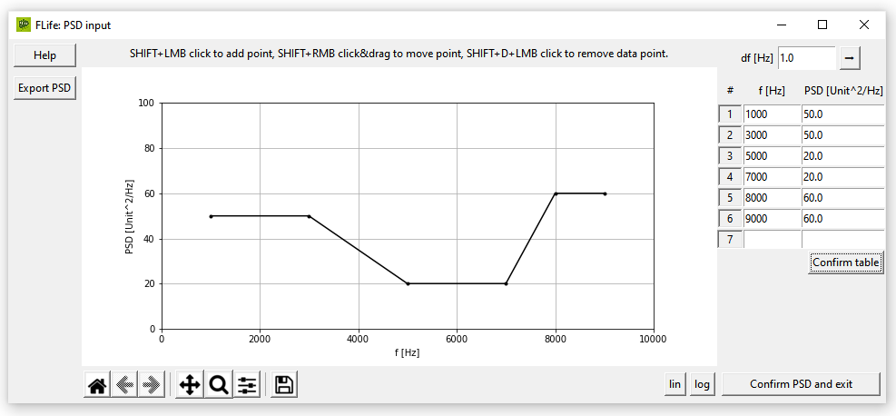
- input = 'GUI' - PSD is provided by user via GUI (graphically and tabulary)
- input = (PSD, freq) - tuple of PSD and frequency vector is provided.
- input = (x, dt) - tuple of time history and sampling period is provided.
sd1 = FLife.SpectralData(input='GUI')
sd2 = FLife.SpectralData()
This is default argument. User is prompted to enter PSD graphically and/or tabulary.
Stationary Gaussian time-history is generated, if parameters T and fs are provided. Otherwise, time-history is generated subsequently, when Rainflow fatigue-life is calculated. Optional parameter for time-history is random generator instance rg (numpy.random._generator.Generator), which determines phase of random process.
seed = 111
rg =  np.random.default_rng(seed)
# time-history can be generated at SpectralData object instantiation. Sampling frequency `fs` and signal length `T` parameter are needed.
sd3 = FLife.SpectralData(input='GUI', T=1, fs=1e5, rg=rg)

time_history = sd3.data
# time-history duration and sampling period are dependent on frequency vector length and step
T = sd3.t # time-history duration
dt = sd3.dt # sampling period
time = np.arange(0, T, dt)
plt.plot(time, time_history)PSD and frequency arrays are given as input. Both arrays must be of type np.ndarray.
Stationary Gaussian time-history is generated, if parameters T and fs are provided. Otherwise, time-history is generated subsequently, when Rainflow fatigue-life is calculated. Optional parameter for time-history is random generator instance rg (numpy.random._generator.Generator), which determines phase of random process.
seed = 111
rg =  np.random.default_rng(seed)
freq = np.arange(0,300)
f_low, f_high = 100, 120
A = 1 # PSD value
PSD = np.interp(freq, [f_low, f_high], [A,A], left=0, right=0) # Flat-shaped one-sided PSD

sd4 = FLife.SpectralData(input = (PSD, freq))
# time-history can be generated at SpectralData object instantiation. Sampling frequency `fs` and signal length `T` parameter are needed.
sd5 = FLife.SpectralData(input = (PSD, freq), T=1, fs=1e5, rg=rg)

time_history = sd5.data
# time-history duration and sampling period are dependent on frequency vector length and step
T = sd5.t # time-history duration
dt = sd5.dt # sampling period
time = np.arange(0, T, dt)
plt.plot(time, time_history)Time history x and sampling period dt are given as input. x must be of type np.ndarray and dt of type float, int.
seed = 111
rg =  np.random.default_rng(seed)
freq = np.arange(0,100)
f_low, f_high = 40, 70
A = 1 # PSD value
PSD = np.interp(freq, [f_low, f_high], [A,A], left=0, right=0) # Flat-shaped one-sided PSD

time, signal = FLife.tools.random_gaussian(freq=freq, PSD=PSD, T=10, fs=1e3, rg=rg)
dt = time[1]

sd6 = FLife.SpectralData(input=(signal,dt))

# Get PSD data from spectralData object
freq = sd6.psd[:,0]
PSD = sd6.psd[:,1]
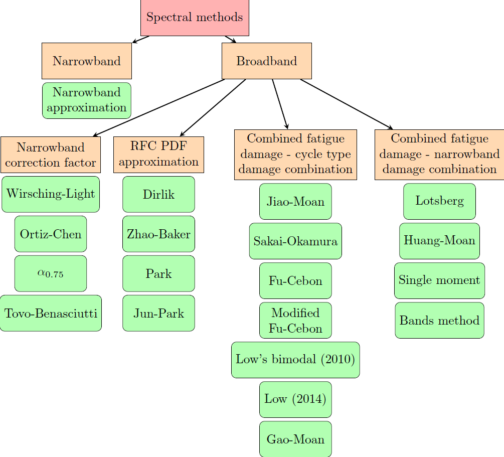
plt.plot(freq, PSD)Currently 20 spectral methods are supported. Methods for broadband process are organized into 4 subgroups:
- Narrowband correction factor; methods are based on narrowband approximation, accounting for broadband procces with correction factor.
- RFC PDF approximation; methods are based on approximation of Rainflow Probability Density Function.
- Combined fatigue damage - cycle damage combination; methods are based on splitting of PSD of broadband process into N narrowband approximations and accounting the formation of distinct categories of cycles.
- Combined fatigue damage - narrowband damage combination; methods are based on splitting of PSD of broadband process into N narrowband approximations and summing narrowband damages by suitable damage conbination rule.
SpectralData instance is prerequisite for spectral method instantiation. For multimodal spectral methods, PSD splitting type can be specified:
- PSD_splitting=('equalAreaBands', N) - PSD is divided into N equal area bands.
- PSD_splitting=('userDefinedBands', [f_1_ub, f_2_ub, ..., f_i_ub, ..., f_N_ub])) - Band upper boundary frequency f_i_ub is taken as boundary between two bands, i.e. i-th upper boundary frequency equals i+1-th lower boundary frequency.
nb = FLife.Narrowband(sd)
dirlik = FLife.Dirlik(sd)
tb = FLife.TovoBenasciutti(sd)
jm1 = FLife.JiaoMoan(sd)
jm2 = FLife.JiaoMoan(sd, PSD_splitting=('equalAreaBands', 2)) # same as jm1, PSD is divided in 2 bands with equal area
jm3 = FLife.JiaoMoan(sd, PSD_splitting=('userDefinedBands', [80,150])) #80 and 150 are bands upper limits [Hz]Some spectral methods supports PDF stress cycle amplitude via get_PDF(s, **kwargs) function:
s = np.arange(0,np.max(x),.001)
plt.plot(s,nb.get_PDF(s), label='Narrowband')
plt.plot(s,dirlik.get_PDF(s), label='Dirlik')
plt.plot(s,tb.get_PDF(s, method='method 2'), label='Tovo-Benasciutti')
plt.legend()
plt.show()
Vibration-fatigue life is returned by function get_life(C,k,**kwargs):
C = 1.8e+22  # S-N curve intercept [MPa**k]
k = 7.3 # S-N curve inverse slope [/]

life_nb = nb.get_life(C = C, k=k)
life_dirlik = dirlik.get_life(C = C, k=k)
life_tb = tb.get_life(C = C, k=k, method='method 1')Vibration-fatigue life can be compared to rainflow method. When Rainflow class is instantiated, time-history is generated and assigned to SpectralData instance, if not already exist. By providing optional parameter rg (numpy.random._generator.Generator instance) phase of stationary Gaussian time history is controlled.
sd = FLife.SpectralData(input='GUI') # time history is not generated at this point

seed = 111
rg =  np.random.default_rng(seed)
rf1 = FLife.Rainflow(sd T=100, fs=1e3) # time history is generated and assigned to parameter SpectralData.data
rf2 = FLife.Rainflow(sd, T=100, fs =1e3,  rg=rg) # time history is generated and assigned to parameter SpectralData.data, signal phase is defined by random generator
rf_life_3pt = rf2.get_life(C, k, algorithm='three-point')
rf_life_4pt = rf2.get_life(C, k, algorithm='four-point', nr_load_classes=1024)

error_nb = FLife.tools.relative_error(life_nb, rf_life_3pt)
error_dirlik = FLife.tools.relative_error(life_dirlik, rf_life_3pt)
error_tb = FLife.tools.relative_error(life_tb, rf_life_3pt)- References:
- Janko Slavič, Matjaž Mršnik, Martin Česnik, Jaka Javh, Miha Boltežar. Vibration Fatigue by Spectral Methods, From Structural Dynamics to Fatigue Damage – Theory and Experiments, ISBN: 9780128221907, Elsevier, 1st September 2020, see Elsevier page.
- Aleš Zorman and Janko Slavič and Miha Boltežar. Vibration fatigue by spectral methods—A review with open-source support, Mechanical Systems and Signal Processing, 2023, see https://doi.org/10.1016/j.ymssp.2023.110149

