SpatialDE

SpatialDE is a method to identify genes which significantly depend on spatial coordinates in non-linear and non-parametric ways. The intended applications are spatially resolved RNA-sequencing from e.g. Spatial Transcriptomics, or in situ gene expression measurements from e.g. SeqFISH or MERFISH.

Additionally, SpatialDE provides automatic expression histology, a method that groups genes into common spatial patterns (and conversely reveal histological patterns based on gene coexpression).

This repository contains both the implementations of our methods, as well as case studies in applying it.

The key features of our method are

Unsupervised - No need to define spatial regions
Non-parametric and non-linear expression patterns
Automatic histology based on spatially coexpressed genes
Extremely fast - Transcriptome wide tests takes only a few minutes on normal computers

The primary implementation is as a Python 3 package, and can be installed from the command line by

$ pip install spatialde

(This should only take a minute or so on a typical system)

To see usage example of SpatialDE either keep reading, or look in the Analysis directory. The following examples are provided:

BreastCancer - Transcriptome wide study on breast cancer tissue from Spatial Transcriptomics.
Frog - A time course of RNA-seq ("1-d space") of Xenopus development.
MERFISH - Expression from single cells in a region of an osteoblast culture using the MERFISH technology with 140 probes.
MouseOB - Spatial Transcriptomics assay of a slice of Mouse Olfactory Bulb. (Also see below).
SeqFISH - Expression counts of single cells from mouse hippocampus using the SeqFISH technology with 249 probes.

If you wish to look at the data used or run the notebooks and scripts from start to finish, the data needs to be fetched using `git lfs <https://git-lfs.github.com/>`__, a plugin to git for managing large files. Installation instructions are available on the projects website. Once git lfs is installed and you have cloned this repository, data can be downloaded by running git lfs pull from inside any repository directory.

Below follows a typical usage example in interactive form.

SpatialDE significance test example use

%pylab inline
import pandas as pd

rcParams['axes.spines.right'] = False
rcParams['axes.spines.top'] = False

import NaiveDE
import SpatialDE

Populating the interactive namespace from numpy and matplotlib

As an example, let us look at spatially dependent gene expression in Mouse Olfactory Bulb using a data set published in Stahl et al 2016. With the authors method, hundrads of locations on a tissue slice can be sampled at once, and gene expression is measured by sequencing in an unbiased whole-transcriptome manner.

counts = pd.read_csv('Analysis/MouseOB/data/Rep11_MOB_0.csv', index_col=0)
counts = counts.T[counts.sum(0) >= 3].T  # Filter practically unobserved genes

print(counts.shape)
counts.iloc[:5, :5]

(262, 14859)

.dataframe tbody tr th:only-of-type { vertical-align: middle; } .dataframe tbody tr th { vertical-align: top; } .dataframe thead th { text-align: right; }

	Nrf1	Zbtb5	Ccnl1	Lrrfip1	Bbs1
16.92x9.015	1	1	1	2	1
16.945x11.075	0	0	3	2	2
16.97x10.118	0	1	1	0	0
16.939x12.132	1	0	1	0	4
16.949x13.055	0	0	0	3	0

sample_info = pd.read_csv('Analysis/MouseOB/MOB_sample_info.csv', index_col=0)
counts = counts.loc[sample_info.index]  # Align count matrix with metadata table

sample_info.head(5)

.dataframe tbody tr th:only-of-type { vertical-align: middle; } .dataframe tbody tr th { vertical-align: top; } .dataframe thead th { text-align: right; }

	x	y	total_counts
16.92x9.015	16.920	9.015	18790
16.945x11.075	16.945	11.075	36990
16.97x10.118	16.970	10.118	12471
16.939x12.132	16.939	12.132	22703
16.949x13.055	16.949	13.055	18641

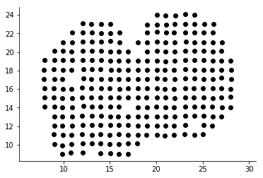
We can plot the x and y coordinates in the sample info table to see which locations of the tissue slice has been sampled.

figsize(6, 4)
plt.scatter(sample_info['x'], sample_info['y'], c='k');
plt.axis('equal');

Our method assumes normally distributed noise, but the data we are using is from expression counts, and empirically seems to follow a negative binomial distribution. We use technique by Anscombe to approximately transform the data to normal distributed noise.

Secondly, library size or sequencing depth of the spatial samples will bias the expression of every gene. We use linear regression to account for this effect before performing the spatial test.

norm_expr = NaiveDE.stabilize(counts.T).T
resid_expr = NaiveDE.regress_out(sample_info, norm_expr.T, 'np.log(total_counts)').T

For the sake of this example, let's just run the test on 1000 random genes. This should just take a few seconds. With our very fast implementation, testing all 14,000 genes takes about 10 minutes.

sample_resid_expr = resid_expr.sample(n=1000, axis=1, random_state=1)

X = sample_info[['x', 'y']]
results = SpatialDE.run(X, sample_resid_expr)

INFO:root:Performing DE test
INFO:root:Pre-calculating USU^T = K's ...
INFO:root:Done: 0.11s
INFO:root:Fitting gene models
INFO:root:Model 1 of 10
INFO:root:Model 2 of 10
INFO:root:Model 3 of 10
INFO:root:Model 4 of 10
INFO:root:Model 5 of 10
INFO:root:Model 6 of 10
INFO:root:Model 7 of 10
INFO:root:Model 8 of 10
INFO:root:Model 9 of 10
INFO:root:Model 10 of 10

The result will be a DataFrame with P-values and other relevant values for each gene.

The most important columns are

g - The name of the gene
pval - The P-value for spatial differential expression
qval - Signifance after correcting for multiple testing
l - A parameter indicating the distance scale a gene changes expression over

results.head().T

.dataframe tbody tr th:only-of-type { vertical-align: middle; } .dataframe tbody tr th { vertical-align: top; } .dataframe thead th { text-align: right; }

	0	1	2	3	4
FSV	0.999955	2.0597e-09	2.0597e-09	2.0597e-09	2.0597e-09
M	4	4	4	4	4
g	2410016O06Rik	Arpp19	Srsf7	Wbp7	Cpsf3l
l	0.402001	0.402001	0.402001	0.402001	0.402001
max_delta	4.53999e-05	4.85165e+08	4.85165e+08	4.85165e+08	4.85165e+08
max_ll	-52.2589	-107.685	-114.477	-112.664	-49.1672
max_mu_hat	-0.826851	-2.21845	-6.67811	-2.25044	0.146089
max_s2_t_hat	0.666985	1.04203e-08	9.22126e-08	1.07257e-08	2.20142e-10
model	SE	SE	SE	SE	SE
n	260	260	260	260	260
s2_FSV	1.94342	0.253788	47.2945	0.363388	4.48293
s2_logdelta	6.81931e+08	4.3315e+16	8.07194e+18	6.20209e+16	7.65119e+17
time	0.00134182	0.00104499	0.000994921	0.000999928	0.00106692
BIC	126.761	237.613	251.196	247.571	120.577
max_ll_null	-53.706	-107.686	-114.478	-112.665	-49.1681
LLR	1.44715	0.000964007	0.000964011	0.000964007	0.00096401
pval	0.228986	0.975231	0.975231	0.975231	0.975231
qval	0.975231	0.975231	0.975231	0.975231	0.975231

results.sort_values('qval').head(10)[['g', 'l', 'qval']]

.dataframe tbody tr th:only-of-type { vertical-align: middle; } .dataframe tbody tr th { vertical-align: top; } .dataframe thead th { text-align: right; }

	g	l	qval
890	Kcnh3	1.907609	0.001512
772	Pcp4	1.135190	0.013843
736	Igfbp2	1.135190	0.013843
800	Gng13	1.907609	0.022632
646	Naaa	0.675535	0.051705
749	Map1b	1.135190	0.051705
826	Gng4	1.907609	0.051705
724	Fmo1	1.135190	0.096710
714	Slc38a3	1.135190	0.096710
712	Hpcal4	1.135190	0.107360

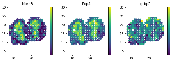
We detected a few spatially differentially expressed genes, Cck and Ptn for example.

A simple way to visualize these genes is by plotting the x and y coordinates as above, but letting the color correspond to expression level.

figsize(10, 3)
for i, g in enumerate(['Kcnh3', 'Pcp4', 'Igfbp2']):
    plt.subplot(1, 3, i + 1)
    plt.scatter(sample_info['x'], sample_info['y'], c=norm_expr[g]);
    plt.title(g)
    plt.axis('equal')


    plt.colorbar(ticks=[]);

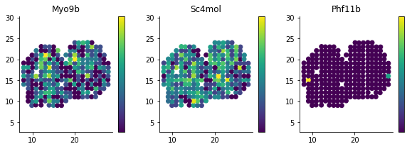
For reference, we can compare these to genes which are not spatially DE

results.sort_values('qval').tail(10)[['g', 'l', 'qval']]

.dataframe tbody tr th:only-of-type { vertical-align: middle; } .dataframe tbody tr th { vertical-align: top; } .dataframe thead th { text-align: right; }

	g	l	qval
334	Tmem70	0.402001	0.975231
335	Rnf20	0.402001	0.975231
336	Zfp85-rs1	0.402001	0.975231
337	C1qtnf7	0.402001	0.975231
338	Ap4b1	0.402001	0.975231
339	Psma4	0.402001	0.975231
340	Aldh3b1	0.402001	0.975231
341	Hdx	0.402001	0.975231
328	Zfp113	0.402001	0.975231
999	Preb	9.052138	0.975231

figsize(10, 3)
for i, g in enumerate(['Myo9b', 'Sc4mol', 'Phf11b']):
    plt.subplot(1, 3, i + 1)
    plt.scatter(sample_info['x'], sample_info['y'], c=norm_expr[g]);
    plt.title(g)
    plt.axis('equal')


    plt.colorbar(ticks=[]);

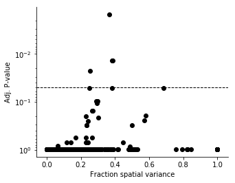
In regular differential expression analysis, we usually investigate the relation between significance and effect size by so called volcano plots. We don't have the concept of fold change in our case, but we can investigate the fraction of variance explained by spatial variation.

figsize(5, 4)
plt.yscale('log')

plt.scatter(results['FSV'], results['qval'], c='black')

plt.axhline(0.05, c='black', lw=1, ls='--');

plt.gca().invert_yaxis();
plt.xlabel('Fraction spatial variance')
plt.ylabel('Adj. P-value');

Automatic expression histology

To perform automatic expression histology (AEH), the genes should be filtered by SpatialDE significance. For this example, let us use a very weak threshold. But in typical use, filter by qval < 0.05

sign_results = results.query('qval < 0.5')

AEH requires two parameters: the number of patterns, and the characteristic lengthscale for histological patterns.

For some guidance in picking the lengthscale l we can look at the optimal lengthscale for the signficant genes.

sign_results['l'].value_counts()

1.135190    11
1.907609     4
0.675535     4
3.205604     1
Name: l, dtype: int64

Here we see that the lengthscale on average is ~1.5, to use some extra spatial covariance, we put this paramater to l = 1.8.

For the number of patterns, we try C = 3.

histology_results, patterns = SpatialDE.aeh.spatial_patterns(X, resid_expr, sign_results, C=3, l=1.8, verbosity=1)

iter 0, ELBO: -9.48e+08
iter 1, ELBO: -4.20e+08, delta_ELBO: 5.28e+08
iter 2, ELBO: -4.20e+08, delta_ELBO: 7.63e+02
iter 3, ELBO: -4.20e+08, delta_ELBO: 2.07e+02
iter 4, ELBO: -4.20e+08, delta_ELBO: 8.03e+01
iter 5, ELBO: -4.20e+08, delta_ELBO: 3.40e+00
iter 6, ELBO: -4.20e+08, delta_ELBO: 6.62e-02
iter 7, ELBO: -4.20e+08, delta_ELBO: 2.75e-03
iter 8, ELBO: -4.20e+08, delta_ELBO: 3.96e-03
iter 9, ELBO: -4.20e+08, delta_ELBO: 7.49e-05
Converged on iter 9

After fitting the AEH model, the function returns two DataFrames, one with pattern membership information for each gene:

histology_results.head()

.dataframe tbody tr th:only-of-type { vertical-align: middle; } .dataframe tbody tr th { vertical-align: top; } .dataframe thead th { text-align: right; }

	g	membership	pattern
564	AI593442	1.0	1
619	Arhgef9	1.0	1
632	6330403K07Rik	1.0	1
646	Naaa	1.0	0
712	Hpcal4	1.0	2

And one with realizations for the underlying expression for each histological pattern.

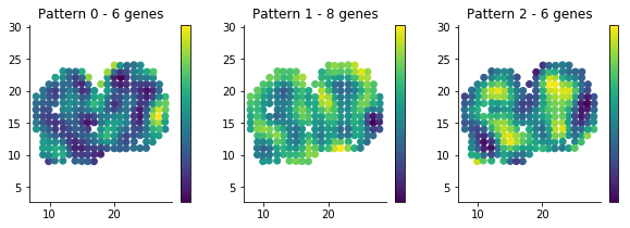
We can visualize this underlying expression in the tissue context as we would for any individual gene.

figsize(10, 3)
for i in range(3):
    plt.subplot(1, 3, i + 1)
    plt.scatter(sample_info['x'], sample_info['y'], c=patterns[i]);
    plt.axis('equal')
    plt.title('Pattern {} - {} genes'.format(i, histology_results.query('pattern == @i').shape[0] ))
    plt.colorbar(ticks=[]);

It is usually interesting to see what the coexpressed genes determining a histological pattern are:

for i in histology_results.sort_values('pattern').pattern.unique():

    print('Pattern {}'.format(i))
    print(', '.join(histology_results.query('pattern == @i').sort_values('membership')['g'].tolist()))
    print()

Pattern 0
Naaa, Aebp1, Mfap3l, Fmo1, 2810002D19Rik, Gng13

Pattern 1
Map2, Arhgef9, AI593442, 6330403K07Rik, Slc38a3, Igfbp2, Nmb, Map1b

Pattern 2
Hpcal4, Snap25, Pcp4, Gng4, Ppfia2, Kcnh3

lambdamoses/SpatialDE

SpatialDE

SpatialDE significance test example use

Automatic expression histology