MDSmonkey

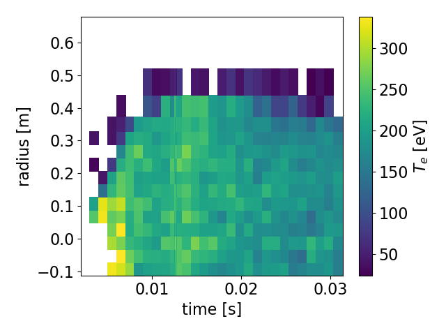
MDSmonkey helps you explore an unfamiliar MDSplus database (tree) and begin analyzing the data in Python, in less than one minute. By using xarray, publication-quality plots can be produced in 6 lines of code:

    > from MDSmonkey import get_tree
    > tree = get_tree(101010,"phys","my.server.com")
    > te = tree.diagnostics.thomson.dts02.te
    > te = te.rename({"dim_0":"time","dim_1":"radius"})
    > te.attrs['long_name'] = r'$T_e$'
    > te.plot()

Tutorial:

This walk-through illustrates a typical workflow when using MDSmonkey to approach an unfamiliar database, find what data is available, and plot it.

Basic access & exploration

The first step is to initialize a tree.

    > from MDSmonkey import get_tree
    > tree = get_tree(101010,"phys","my.server.com")
    > tree
    
    Branch \phys : number of subnodes: 14
    _____________________________________
    fueling     : Branch : number of subnodes: 4
    physics     : Branch : number of subnodes: 39
    vacuum      : Branch : number of subnodes: 15
    viz_only    : Branch : number of subnodes: 17
    electrodes  : Branch : number of subnodes: 6
    ...

Note that the ellipsis is just for the documentation, in reality all Branches will be shown.

If you are using iPython, you can see the branches by typing tree.<tab>, which will display a drop-down list of the branches. Use the up/down arrows and hit enter to select. Typing tree.p<tab> will display a list a sublist, or in this case will autocomplete to tree.physics because there is only one item starting with p.

The tree is nested. Each node (Branch or Leaf) may have both Leafs (which have data attributes) and Branches (which do not). Each node displays its path name (ex: \phys::top.physics) when printed. Branches display their type, path, and a short description of the of the subnodes below them. Leafs display their type, path, and length (in bytes) of their data, along with a short description of the subnodes below them (if any).

Note that by default, the trim_dead_branches feature of get_tree is used. This removes any Branch that does not have a Leaf with a non-zero amount of data as a descendant. Checking the length slows the initialization considerably (~20 seconds vs ~1 second, depending on the size of the database). If you are in a hurry, you can supply the optional trim_dead_branches=False argument to get_tree.

    > tree.physics
    
    Branch \phys::top.physics : number of subnodes: 39
    __________________________________________________
    b0          : Leaf : number of subnodes: 4
    b0_avg      : Leaf : number of subnodes: 4
    be_max      : Leaf : number of subnodes: 4
    be_z0       : Leaf : number of subnodes: 4
    e_th        : Leaf : number of subnodes: 4
    ...

Let's have a look at the data of the Leaf called be_max:

    > tree.physics.be_max
    
    Leaf \PHYS::B0 : length of data: 734 bytes
    __________________________________________
    data_err   : Leaf : number of subnodes: 0
    data_err_h : Leaf : number of subnodes: 0
    data_err_l : Leaf : number of subnodes: 0
    description: Leaf : number of subnodes: 0

Because be_max is a Leaf it has a data attribute. When introspecting this attribute, the data is loaded at this time from the tree (there may be a pause).

    > tree.physics.be_max.data

    <xarray.DataArray 'BE_MAX' (dim_0: 94999)>
    array([0.08225632, 0.08221801, 0.08222205, ..., 0.0775292 , 0.07756143,
           0.07744625], dtype=float32)
    Coordinates:
      * dim_0    (dim_0) float64 -0.0004996 -0.0004992 -0.0004988 ... 0.0375 0.0375
    Attributes:
        units:    T

The xarray.DataArray type knows how to plot itself nicely.

    > tree.physics.be_max.data.plot()

Combining nodes into a single array or dataset

Sometimes diagnostic channels are broken up into different nodes instead of being represented as a single multi-dimensional array.

    > ndl = tree.diagnostics.thomson.dts02.ndl
    > ndl
    
    Branch \phys::top.diagnostics.thomson.dts02.ndl : number of subnodes: 14
    ________________________________________________________________________
    ndl_01: Leaf : number of subnodes: 4
    ndl_02: Leaf : number of subnodes: 4
    ndl_03: Leaf : number of subnodes: 4
    ndl_04: Leaf : number of subnodes: 4
    ndl_05: Leaf : number of subnodes: 4
    ...

We can handle this situation using the concat keyword to the diagnosticXarray function. The data of each 1D Leaf is stacked into a new 2D array indexed by channel.

    > from MDSmonkey import diagnosticXarray
    > ndlarray = diagnosticXarray(ndl,behavior='concat')
    > ndlarray 
        
        <xarray.DataArray 'NDL_DTS02_01' (channel: 14, dim_0: 34)>
    array([[          nan, 1.6703393e+18, 1.3293034e+18, 1.5485215e+18,
            1.7731074e+18, 2.2600095e+18, 4.0675737e+18, 2.2424507e+18,   
    ...
            3.1138925e+18, 3.2072900e+18, 2.9299945e+18, 3.1664352e+18,
            3.0876216e+18, 3.2820408e+18]], dtype=float32)
    Coordinates:
      * dim_0    (dim_0) float32 0.0025 0.0035 0.0045 ... 
      * channel  (channel) <U6 'ndl_01' 'ndl_02' 'ndl_03' ... 
    Attributes:
        units:    1/m^2

In some cases, a diagnostic has heterogeneous data types. For instance, the Thomson ne,te (electron temperature & density) belong in the same dataset because they share the same dimensions, but they are not part of the same array because they are not the same kind of quantity & have separate units. So, we use merge behavior for this kind of information gathering.

    > ts = tree.diagnostics.thomson.dts02
    > ts
    
    Branch \phys::top.diagnostics.thomson.dts02 : number of subnodes: 6
    ___________________________________________________________________
    laser_energy: Leaf : number of subnodes: 4
    ne          : Leaf : number of subnodes: 4
    te          : Leaf : number of subnodes: 4
    te_max      : Leaf : number of subnodes: 4
    apd_monitors: Branch : number of subnodes: 2
    ndl         : Branch : number of subnodes: 14
    
    > tsarr = diagnosticXarray(ts,subset=['ne','te'],behavior='merge')
    > tsarr 
    
    <xarray.Dataset>
    Dimensions:   (dim_0: 34, dim_1: 16)
    Coordinates:
      * dim_0     (dim_0) float32 0.0025 0.0035 0.0045 ... 0.029859 0.030859
      * dim_1     (dim_1) float32 -0.0933 -0.0533 -0.0133 ... 0.4792 0.5592 
    Data variables:
        ne  (dim_1, dim_0) float32 nan nan nan 4.2912584e+18 ... 
        ne  (dim_1, dim_0) float32 nan nan nan 331.0 317.0 ...

Adding supplementary information

Unfortunately MDSplus does not support dimension names so, they cannot be made available automatically -- the user needs to obtain this information by some other means. Once you know the dimension names, you can add them like this:

    > tsarr = tsarr.rename({"dim_0":"time","dim_1":"radius"})
    > tsarr
    
    <xarray.Dataset>
    Dimensions:   (radius: 16, time: 34)
    Coordinates:
      * time      (time) float32 0.0025 0.0035 0.0045 ... 0.028859 0.029859 
      * radius    (radius) float32 -0.0933 -0.0533 -0.0133 ... 0.4792 0.5592 
    Data variables:
        ne  (radius, time) float32 nan nan nan 4.2912584e+18 ... nan nan
        te  (radius, time) float32 nan nan nan 331.0 317.0 ... nan nan

Another fancy feature is long_name attributes, which can be used to give LaTeX-style mathematical expressions for titling the plots.

    >tsarr.time.attrs['long_name'] = r'$\Delta t$'
    >tsarr.radius.attrs['long_name'] = r'$r_{major}$'
    >tsarr.ne.attrs['long_name'] = r'$n_{e}$'
    >tsarr.te.attrs['long_name'] = r'$T_{e}$'

Basic analysis and plotting

We can plot this data in several ways: as profiles at particular times or at all times together, or as traces over time at particular radii (or all radii), or we can make a 2D heatmap.

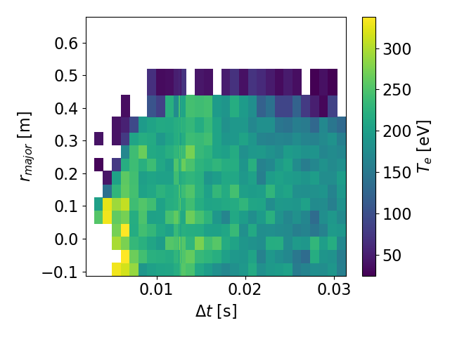
    >tsarr.te.plot()  #2D heatmap
    
    >tsarr.te.plot(x='radius') #Transpose the axes
    
    >tsarr.te.sel(time=16.6e-3,method='nearest').plot()  #profile at the time closest to 16.6 ms
    
    >tsarr.te.sel(time=slice(16.5e-3,20.5e-3)).plot() #2D heatmap over a shorter range
    
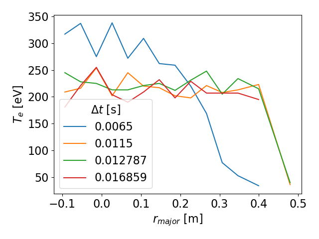
    >tsarr.te.sel(time=slice(5.5e-3,20.5e-3,5)).plot(hue='time') #series of 1D radial profiles colored by time
    
    >tsarr.te.isel(time=12).plot() #1D profile at the 12th time point
    
    >tsarr.te.mean(dim='time').plot() #Plot the time-averaged profile

Sample 2D heatmap. Notice how the colorbar, x-axis, and y-axis automatically have their names and units attached (if the units are available.) The fancy long_names we gave are rendered nicely as well.

Sample 1D profile series. Note how the legend automatically shows the time of each slice.

Save and restore data

It is also possible to save & reload data to an HDF5 file:

    import xarray as xr
    > tsarr.to_netcdf("my_filename_for_ts.h5")
    > tsarr_reloaded = xr.load_dataset("my_filename_for_ts.h5")

About the project

I (@lamorton) wrote this because I've worked with >4 different devices (MST, NSTX/NSTX-U, DIII-D, C-2W). Finding out what data is available and where has generally been a chore each time. The goal of MDSmonkey was to have a tool that I could reuse for the N+1th device. It's intended for students or postdocs who need to hit the ground running.

Key features:

Exploration: see all the branches in the tree that contain data items.
Tidiness: by default, 'prunes' away branches that do not contain data, for an uncluttered view.
Speed: data is loaded only when needed, and cached for reuse.
Conciseness: absolute minimum of boilerplate required to get nice plots.
Generality: works for any MDSplus installation. No customization required.
Unification: find, plot, and do math on the data with one tool.

Key non-features:

Database editing: does not write data or construct a tree. Meant for analysis.
Liveness: does not have live updates as data comes in from a shot. Meant for post-shot analysis.
Customization: does not supply machine-specific defaults. Meant for robust generality.
Artificial intelligence: does not infer anything (like dimension names). Meant to reflect exactly what exists in the database.
Graphical interface: this tool use the iPython interpreter as the user interface.

Possible eventual features:

Multishot interface: presently, each shot needs a separate tree instance, because the shape of the tree and the shape of the data records may change shot-to-shot. It may be possible to circumvent these restrictions and enable a single tree to contain multi-shot data.

Tools with overlapping scope:

jScope/dwScope: GUIs with live updating plots of data (can't do math or explore the tree).
traverser: GUI for looking at / editing the tree (can't plot the data, nor prune 'dead' branches).
Fusion Data Platform: very similar to MDSmonkey. Provides a standardized interface to multiple machines, using JSON templates that must be written for each one.
OMFIT: Has MDSplus support for some machines, with Scope, Profile, and EFIT GUIs

Dependencies:

django
MDSplus
xarray

lamorton/MDSmonkey