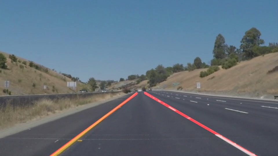
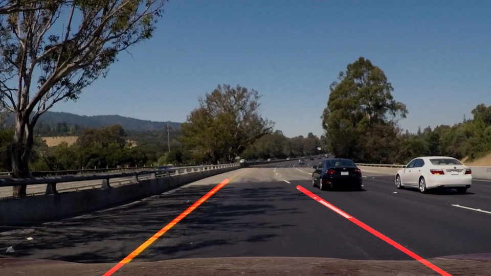
The goals / steps of this project are the following:
- Make a pipeline that finds lane lines on the road
- Reflect on your work in a written report
1. Describe your pipeline. As part of the description, explain how you modified the draw_lines() function.
My pipeline resembles the solution to the lane finding quiz, with the following steps:
- Grayscale - highlight objects based on brightness contrast
- Gaussian Blur - noise reduction
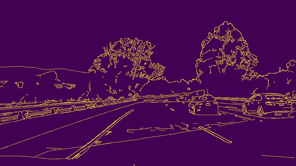
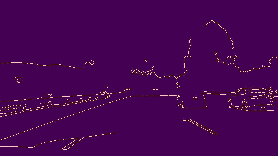
- Canny Edge Detection - detect edges in the image
- Mask Image with Polygon - select an area of interest in the image
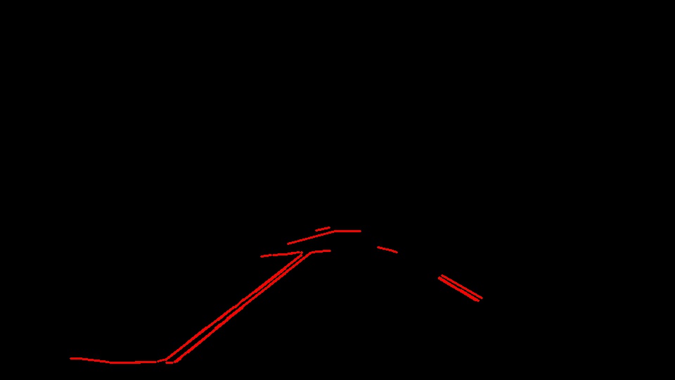
- Hough Transform - average/extrapolate edges into left and right lane lines
Most of the steps above rely on calling library methods or helper functions predefined in the assignment.
In extrapolating the edges into lane lines, I refer to Peteris Rocks's blog post where I first categorize the edges into two groups: positive and negative slope, then I dissemble all the edges into points in the image space and find the line of best fit through each group of points. The result is two lines of best fitting the set of positive slope edges (that line will be the right lane line) and set of negative slope edges (left lane line).
(These two lines of best fit are a function that behaves mathematically like y = mx + b)
To draw the two lane lines on the image, I identify the start and stop coordinates for the line.
      (x_end_l, y_end_l)    (x_start_r, y_start_r)
                   *           *
                  /             \
        Left     /               \     Right
        Lane    /                 \    Lane
               /                   \
              *                     *
(x_start_l,y_start_l)         (x_end_r, y_end_r)
Recall that the line of best fit found earlier is a function takes in an x-coordinate and return the y-coordinate. To find the start and stop coordinates, I have to identify the starting and ending x-coordinate (x_start and x_end), and plug the x-coordinates into the line of best fit to get the y-coordinates (y_start and y_end)
For the left lane line, x_start_l will be 0 (leftmost of the image) and x_end_l will be the maximum x-coordinate in the set of negative slope edges (in order words, the rightmost x-coordinate in all the left lane line edges).
Similarly, for the right lane line, x_start_r will be the minimum x-coordinate in the set of positive slope edges and x_end_r will be the width of the image (rightmost x-coordinate of the image).
The result of this approach works fine for the example videos and images, fails to identify the lane lines in the challenge video.
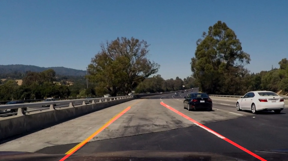
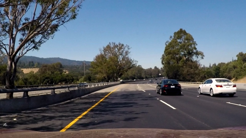
I extract two key frames from the challenge video that poses a challenge to the processing:
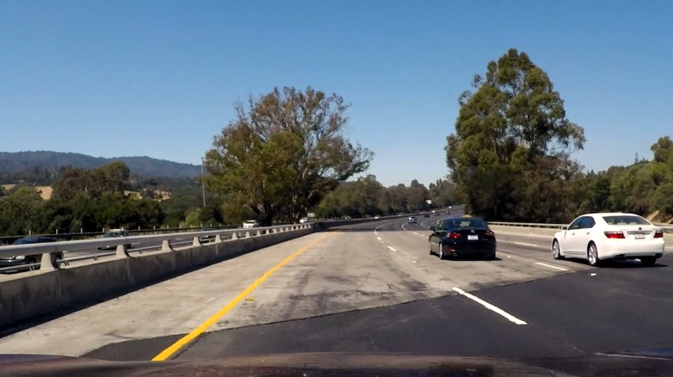
The bright color of the cement obscures the yellow lane in a grayscale image.
To address the issues, I reanalyze the image in the three color channel: red, green and blue in addition to the grayscale channel.
On the other hand the shadow casting from the trees on the side and the uneven surface on the road create noises on the ground.
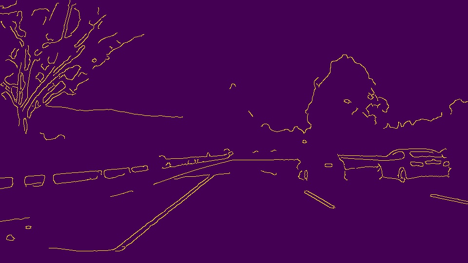
To remove the false positive edges, I filter out the edges with flat slope < 0.5.
Although the techniques mention above resolves some of the issues in the challenge video, the pipeline is very vulnerable to noise. It is not robust enough to distinguish shadows and edges of road pavement blocks from lane lines. If a yellowish or whitish object enters the masked area in the image, they can be false positive lane lines.
The current solution only works on specific road conditions. A snowing day will make matters worse as pile of snow could misinterpreted as lanes. Simply having a white car at the front of the image could undo all efforts attempted in this assignment.
In addition to analyze the image in multiple color channels, I could possibly improve lane finding by selecting objects in the image of a specific color, like yellow or white.
Nevertheless, the current approach to lane finding is still insufficient. We need to be able to recognize different objects in the image and distinguish different objects perhaps through use of deep neutral nets.
