findiff

A Python package for finite difference numerical derivatives and partial differential equations in any number of dimensions.

Features

Differentiate arrays of any number of dimensions along any axis with any desired accuracy order
Accurate treatment of grid boundary
Includes standard operators from vector calculus like gradient, divergence and curl
Can handle uniform and non-uniform grids
Can handle arbitrary linear combinations of derivatives with constant and variable coefficients
Fully vectorized for speed
Calculate raw finite difference coefficients for any order and accuracy for uniform and non-uniform grids
New in version 0.7: Generate matrix representations of arbitrary linear differential operators
New in version 0.8: Solve partial differential equations with Dirichlet or Neumann boundary conditions

Installation

pip install findiff

Derivatives

findiff works in any number of dimensions. But for the sake of demonstration, suppose you want to differentiate a four-dimensional function given on a 4D array f with coordinates x, y, z, u.

For , where x denotes the 0-th axis, we can write

# define operator
d_dx = FinDiff(0, dx)

# apply operator
df_dx = d_dx(f)
# df_dx is now an array of the same shape as f containing the partial derivative

The partial derivative , where z means the 2nd axis, is

d_dz = FinDiff(2, dz)
df_dz = d_dz(f)

Higher derivatives like or can be defined like this:

# the derivative order is the third argument
d2_dx2 = FinDiff(0, dx, 2)
d2f_dx2 = d2_dx2(f)

d4_dy4 = FinDiff(1, dy, 4)
d4f_dy4 = d4_dy4(f)

Mixed partial derivatives like or

d2_dxdz = FinDiff((0, dx), (2, dz))
d2_dxdz(f)

d3_dx2dz = FinDiff((0, dx, 2), (2, dz))

Linear combinations of differential operators like

can be written as

from numpy import meshgrid, sin
X, Y, Z, U = meshgrid(x, y, z, u, indexing="ij")
diff_op = Coef(2*X) * FinDiff((0, dz, 2), (2, dz, 1)) + Coef(3*sin(Y)*Z**2) * FinDiff((0, dx, 1), (1, dy, 2))

Chaining differential operators is also possible, e.g.

diff_op = (FinDiff(0, dx) - FinDiff(1, dy)) * (FinDiff(0, dx) + FinDiff(1, dy))
# is equivalent to
diff_op2 = FinDiff(0, dx, 2) - FinDiff(1, dy, 2)

Standard operators from vector calculus like gradient, divergence and curl are also available, for example:

grad = Gradient(h=[dx, dy, dz, du])
grad_f = grad(f)

More examples can be found here and in this blog.

Derivatives in N dimensions

The package can work with any number of dimensions, the generalization of usage is straight forward. The only limit is memory and CPU speed.

Accuracy Control

When constructing an instance of FinDiff, you can request the desired accuracy order by setting the keyword argument acc.

d2_dx2 = findiff.FinDiff(0, dy, 2, acc=4)
d2f_dx2 = d2_dx2(f)

If not specified, second order accuracy will be taken by default.

Finite Difference Coefficients

Sometimes you may want to have the raw finite difference coefficients. These can be obtained for any derivative and accuracy order using findiff.coefficients(deriv, acc). For instance,

import findiff
coefs = findiff.coefficients(deriv=2, acc=2)

gives

{ 'backward': {'coefficients': array([-1.,  4., -5.,  2.]),
               'offsets': array([-3, -2, -1,  0])},
  'center': {'coefficients': array([ 1., -2.,  1.]),
             'offsets': array([-1,  0,  1])},
  'forward': {'coefficients': array([ 2., -5.,  4., -1.]),
              'offsets': array([0, 1, 2, 3])}
              }

FinDiff operators will use central coefficients whenever possible and switch to backward or forward coefficients if not enough points are available on either side.

If you need exact values instead of floating point numbers, you can request a symbolic solution, e.g.

import findiff
coefs = findiff.coefficients(deriv=3, acc=4, symbolic=True)

gives

{'backward': {'coefficients': [15/8, -13, 307/8, -62, 461/8, -29, 49/8],
              'offsets': [-6, -5, -4, -3, -2, -1, 0]},
 'center': {'coefficients': [1/8, -1, 13/8, 0, -13/8, 1, -1/8],
            'offsets': [-3, -2, -1, 0, 1, 2, 3]},
 'forward': {'coefficients': [-49/8, 29, -461/8, 62, -307/8, 13, -15/8],
             'offsets': [0, 1, 2, 3, 4, 5, 6]}}

If you want to specify the detailed offsets instead of the accuracy order, you can do this by setting the offset keyword argument:

import findiff
coefs = findiff.coefficients(deriv=2, offsets=[-2, 1, 0, 2, 3, 4, 7], symbolic=True)

The resulting accuracy order is computed and part of the output:

{'coefficients': [187/1620, -122/27, 9/7, 103/20, -13/5, 31/54, -19/2835], 
 'offsets': [-2, 1, 0, 2, 3, 4, 7], 
 'accuracy': 5}

Matrix Representation

For a given FinDiff differential operator, you can get the matrix representation using the matrix(shape) method, e.g.

x = [np.linspace(0, 6, 7)]
d2_dx2 = FinDiff(0, x[1]-x[0], 2)
u = x**2

mat = d2_dx2.matrix(u.shape)  # this method returns a scipy sparse matrix
print(mat.toarray())

has the output

[[ 2. -5.  4. -1.  0.  0.  0.]
 [ 1. -2.  1.  0.  0.  0.  0.]
 [ 0.  1. -2.  1.  0.  0.  0.]
 [ 0.  0.  1. -2.  1.  0.  0.]
 [ 0.  0.  0.  1. -2.  1.  0.]
 [ 0.  0.  0.  0.  1. -2.  1.]
 [ 0.  0.  0. -1.  4. -5.  2.]]

The same works for differential operators in higher dimensions. Of course, you can use this matrix to perform the differentiation manually by matrix-vector multiplication:

d2u_dx2 = mat.dot(u.reshape(-1))

Examples using the matrix representation like solving the Schrödinger equation can be found in this blog.

Stencils

You can also take a look at the finite difference stencils, e.g. for a 2D grid:

import numpy as np
from findiff import FinDiff

x, y = np.linspace(0, 1, 100)
X, Y = np.meshgrid(x, y, indexing='ij')
u = X**3 + Y**3
laplace_2d = FinDiff(0, x[1]-x[0], 2) + FinDiff(1, y[1]-y[0], 2)

stencil = laplace_2d.stencil(u.shape)

print(stencil)

yields the following output

('L', 'L'):	{(0, 0): 4.0, (1, 0): -5.0, (2, 0): 4.0, (3, 0): -1.0, (0, 1): -5.0, (0, 2): 4.0, (0, 3): -1.0}
('L', 'C'):	{(0, 0): 0.0, (1, 0): -5.0, (2, 0): 4.0, (3, 0): -1.0, (0, -1): 1.0, (0, 1): 1.0}
('L', 'H'):	{(0, 0): 4.0, (1, 0): -5.0, (2, 0): 4.0, (3, 0): -1.0, (0, -3): -1.0, (0, -2): 4.0, (0, -1): -5.0}
('C', 'L'):	{(-1, 0): 1.0, (0, 0): 0.0, (1, 0): 1.0, (0, 1): -5.0, (0, 2): 4.0, (0, 3): -1.0}
('C', 'C'):	{(-1, 0): 1.0, (0, 0): -4.0, (1, 0): 1.0, (0, -1): 1.0, (0, 1): 1.0}
('C', 'H'):	{(-1, 0): 1.0, (0, 0): 0.0, (1, 0): 1.0, (0, -3): -1.0, (0, -2): 4.0, (0, -1): -5.0}
('H', 'L'):	{(-3, 0): -1.0, (-2, 0): 4.0, (-1, 0): -5.0, (0, 0): 4.0, (0, 1): -5.0, (0, 2): 4.0, (0, 3): -1.0}
('H', 'C'):	{(-3, 0): -1.0, (-2, 0): 4.0, (-1, 0): -5.0, (0, 0): 0.0, (0, -1): 1.0, (0, 1): 1.0}
('H', 'H'):	{(-3, 0): -1.0, (-2, 0): 4.0, (-1, 0): -5.0, (0, 0): 4.0, (0, -3): -1.0, (0, -2): 4.0, (0, -1): -5.0}

This is a dictionary with the characteristic points as keys and the stencils as values. The 2D grid has 3**2 = 9 "characteristic points", so it has 9 stencils.

'L' stands for 'lowest index' (which is 0), 'H' for 'highest index' (which is the number of points on the given axis minus 1) and 'C' for 'center', i.e. a grid point not at the boundary of the axis.

In 2D the characteristic points are center points ('C', 'C'), corner points: ('L', 'L'), ('L', 'H'), ('H', 'L'), ('H', 'H') and edge-points (all others). For N > 2 dimensions the characteristic points are 3**N analogous tuples with N indices each.

Each stencil is a dictionary itself with the index offsets as keys and the finite difference coefficients as values.

In order to apply the stencil manually, you can use

lap_u = stencil.apply_all(u)

which iterates over all grid points, selects the right right stencil and applies it.

Partial Differential Equations

findiff can be used to easily formulate and solve partial differential equation problems

where L is a general linear differential operator.

In order to obtain a unique solution, Dirichlet, Neumann or more general boundary conditions can be applied.

Boundary Value Problems

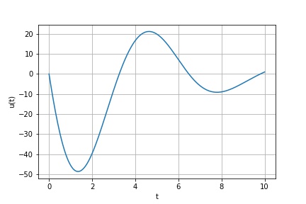
Example 1: 1D forced harmonic oscillator with friction

Find the solution of

subject to the (Dirichlet) boundary conditions

from findiff import FinDiff, Id, PDE

shape = (300, )
t = numpy.linspace(0, 10, shape[0])
dt = t[1]-t[0]

L = FinDiff(0, dt, 2) - FinDiff(0, dt, 1) + Coef(5) * Id()
f = numpy.cos(2*t)

bc = BoundaryConditions(shape)
bc[0] = 0
bc[-1] = 1

pde = PDE(L, f, bc)
u = pde.solve()

Result:

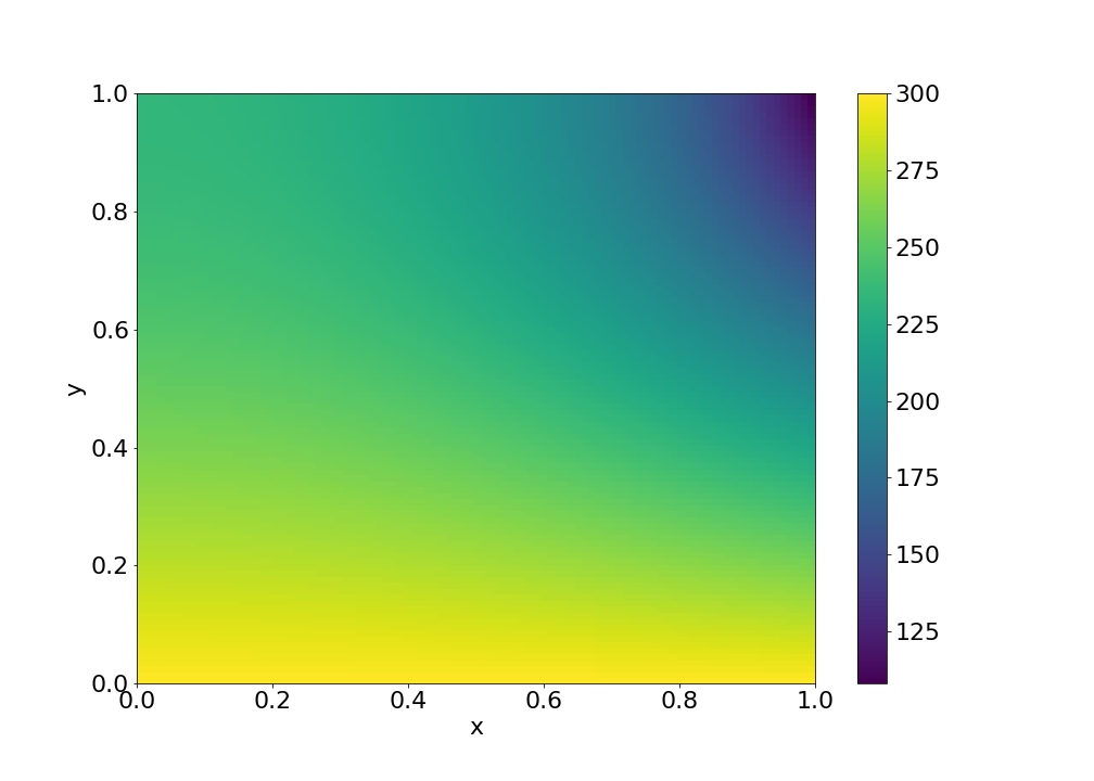
Example 2: 2D heat conduction

A plate with temperature profile given on one edge and zero heat flux across the other edges, i.e.

with Dirichlet boundary condition

and Neumann boundary conditions

shape = (100, 100)
x, y = np.linspace(0, 1, shape[0]), np.linspace(0, 1, shape[1])
dx, dy = x[1]-x[0], y[1]-y[0]
X, Y = np.meshgrid(x, y, indexing='ij')

L = FinDiff(0, dx, 2) + FinDiff(1, dy, 2)
f = np.zeros(shape)

bc = BoundaryConditions(shape)
bc[1,:] = FinDiff(0, dx, 1), 0  # Neumann BC
bc[-1,:] = 300. - 200*Y   # Dirichlet BC
bc[:, 0] = 300.   # Dirichlet BC
bc[1:-1, -1] = FinDiff(1, dy, 1), 0  # Neumann BC

pde = PDE(L, f, bc)
u = pde.solve()