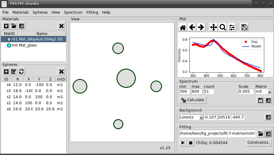
The project was initially developed as a Python wrapper for Multiple Sphere T-Matrix (MSTM) code for the calculation of extinction spectra of nanoparticle aggregates.
Based and inspired by MSТM GUI code https://git.stim.ee.uh.edu/optics/mstm-gui.git by David Mayerich.
MSTM code was published by Dr. Daniel Mackowski and Dr. Michael Mishchenko in: "A multiple sphere T-matrix Fortran code for use on parallel computer clusters," Journal of Quantitative Spectroscopy and Radiative Transfer (2011) 112 2182-2192 [doi].
The MSTM Studio presents several other features, extending the functionality of MSTM.
- Interactive graphical user interface (GUI)
- Alternative Python scripting (more flexible than GUI)
- Mie theory calculations for isolated spherical nanoparticles
- Isolated spheroidal nanoparticles using SpheroidPy
- MSTM calculations for interacting spherical nanoparticles
- Near-field calculation with MSTM
- Materials (dielectric functions): tabulated file, numpy array or analytical expression of Rioux et al [doi] for Au-Ag
- Size-corrected dielectric functions, instances for Au and Ag
- Additional simple spectral shapes (linear, lorentzian, gaussian functions)
- Fitting to experimental data by the mentioned contributions
-
source distribution is available through PyPi repository. Install system-wide by command
pip3 install mstm_studioor for current user by commandpip3 install mstm_studio --user. -
MSTM binary should be compiled and specified by environmental variable
MSTM_BIN. MSTM source and binaries can be obtained on MSTM website. Compiled binaries for Linux Debian x64 and Windows x32 can be found in latest release.
Tested in i) Python3 under Debian10 Linux; ii) Anaconda Python3 under Windows7.
- Python3
- NumPy - numerical python library
- SciPy - scientific python library
Optional
- MatPlotLib - plotting with python
- tkinter, PIL - tk libraries and Python image - for GUI
- ScatterPy - non-spherical particles (spheroids)
Avakyan Leon laavakyan@sfedu.ru, students: Skidanenko Anna (PhD), Yablinovski Kirill (MS), Kostulin Denis (BS).
Under Linux can be run by python3 -m mstm_studio command.
Under Windows the following shell script may be used
@ECHO OFF
PATH=C:\ProgramData\Anaconda3;C:\ProgramData\Anaconda3\Library\mingw-w64\bin;C:\ProgramData\Anaconda3\Library\usr\bin;C:\ProgramData\Anaconda3\Library\bin;C:\ProgramData\Anaconda3\Scripts;C:\ProgramData\Anaconda3\bin;C:\ProgramData\Anaconda3\condabin;%PATH%
set MSTM_BIN="C:\Users\L\Desktop\mstm_studio old\mstm-spectrum\mstm.exe"
python.exe -m mstm_studio
PAUSE
In this script the PATH variable is updated to ensure python binary is in it.
Next, MSTM_BIN environmental variable is set.
Without MSTM the code will work in part, i.e. resctricted to Mie and simple functional (Gauss, Lorentz) contributions.
Alternatively, the python scripting way may be used, which gives full control over the calculations.
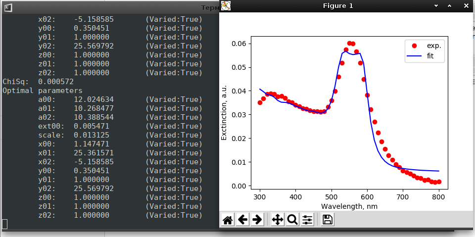
Example script with fitting of experimental data by spheres of material with dielectric function specified in file.
from mstm_studio.fit_spheres_optic import Fitter
from mstm_studio.contributions import ConstantBackground
from mstm_studio.mstm_spectrum import ExplicitSpheres


fitter = Fitter(exp_filename='experiment.dat')   # load experiment
fitter.set_matrix(1.5)  # glass environment
fitter.set_extra_contributions([
    ConstantBackground(wavelengths=fitter.wls)
    ])
# initial configuration: three golden spheres at (0,0,0), (25,0,0) and (0,25,0) with radii 10.
spheres = ExplicitSpheres(N=3, Xc=[0,25,0], Yc=[0,0,25], Zc=[0,0,0], a=[10,10,10], mat_filename='etaGold.txt')
fitter.set_spheres(spheres)

# run fit (takes about a hour)
fitter.run()

fitter.report_result()


# plot results
import matplotlib.pyplot as plt
plt.plot(fitter.wls, fitter.exp, 'ro',
         fitter.wls, fitter.calc, 'b-')
plt.xlabel('Wavelength, nm')
plt.ylabel('Exctinction, a.u.')
plt.show()If you found the code useful please cite following reference:
L. Avakyan, M. Heinz, A. Skidanenko, K. Yablunovskiy, J. Ihlemann, J. Meinertz, C. Patzig, M. Dubiel, L. Bugaev J. Phys.: Condens. Matter (2018) 30 045901 [doi]
If used MSTM you should cite above mentioned Mackowski&Mishchenko paper:
D. Mackowski, M. Mishchenko Journal of Quantitative Spectroscopy and Radiative Transfer (2011) 112 2182-2192 [doi]

