The aims of our analysis are three-fold:
-
To generate an updated estimate on the number of Opportunity Youth in South King County
-
To gain a deeper understanding of the two defining characteristics of Opportunity Youth: education and employment.
-
To observe any trends between the 2016 "Opportunity Youth in the Road Map Project Region" report and the data we are reporting on from 2017.
The Opportunity Youth population is defined as persons aged between 16 and 24 who are not in school and are not working. Throughout this analysis, you may see Opportunity Youth referred to as 'OY'.
We define anyone who is either working or participating in school as Non-Opportunity Youth.
For the purposes of this report, South King County has been defined using the PUMA codes as per the data from the ACS website. After refining the data from the puma_names_2010 table down to King County, the regions which identified 'South' in their puma name was assumed to be apart of South King County. Thus, the PUMA codes we used to define our data set were: 11612, 11613, 11614, 11615
- Throughout this analysis, comparisons are sometimes drawn between this report and the 2016 report on Opportunity Youth. It is important to note that the way the data was defined for the 2016 report differs from how we have defined our data. The 2016 report includes some data from the wider King County area whereas we have stayed strictly within the four aforementioned PUMA codes.
- The 2016 report uses data from the 2014 PUMS data (collected in the 2010 census).
- Our 2020 report utilises data from the 2017 PUMS data, as provided by the ACS website.
- The 2017 PUMS data represents a sample of the population. The ACS included person weightings to allow for appropriate scaling. Numbers quoted in relation to population counts throughout the analysis are based on the person weights.
This analysis was completed in four stages:
-
A map was generated to help visualise the part of King County that are a part of South King County.
-
An updated estimate of the number of Opportunity Youth in South King County as well as a breakdown of this count by age group, PUMA code, educational attainment and employment availability.
-
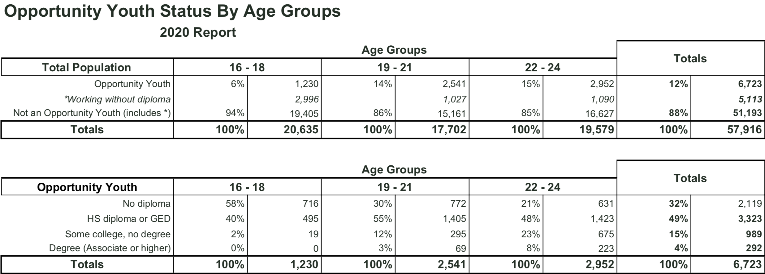
An update of the table "Opportunity Youth Status by Age" from the 2016 report "Opportunity Youth in the Road Map Project Region".
-
A visualisation highlighting a trend between the 2014 data and the current 2017 data.
├── notebooks
│   ├── exploratory (contains all exploratory notebooks)
│   └── report (contains final report notebooks)
├── references
├── reports (contains final README.md file)
│   └── figures (contains figures of visualisations used throughout)
├── src
│   ├── data
│   │   ├── sql
│   ├── data_cleaning (contains .py file of functions used throughout)
│   └── requirements
To begin the analysis of the South King County (SKC) and the Opportunity youth (OY) within SKC we first needed to identify these two parameters. Starting with SKC we are looked at the 2010 Public Use Micro Area (PUMA) codes to see how the census determined south and King County (KC). Using this information and along with the Public Use Microdata Samples (PUMS) we filtered through the geographic locations considered south by the census and matched those corresponding areas with their respective PUMA codes. Now understanding where our OP are located and what area of KC we are looking at we then needed a way to represent this data visually. To do this we utilized GIS oranizations shapefiles and the Geopandas library. After plotting the shapefile for KC, it was then time to create SKC plot that would overlay the KC visual. To do this we utilized the prior mentioned PUMA codes to isolate the specific areas considered South. After that was completed SKC a figure was used as an overlay to then create the entire SKC graph.
In Part 2 of this analysis, we find an updated estimate on the number of Opportunity Youth in South King County.
We will then dive deeper into this population by breaking down the number of Opportunity Youth by puma code, age groups, educational attainment and employment availability.
Using the person weights from the 2017 pums data, we found an updated estimate of the Opportunity Youth in South King County to be 6723.
We can see the breakdown of the OY population by PUMA codes, as per our definition of South King County from Part 1:
-
PUMA 11612 - King County (Far Southwest): 1977 - 29%
-
PUMA 11613 - King County (Southwest Central): 2006 - 30%
-
PUMA 11614 - King County (Southwest): 1530 - 23%
-
PUMA 11615 - King County (Southeast): 1210 - 18%
This distribution of the OY population might lead to further investigations about why the Southwest regions of King County account for 82% of the OY population in South King County. What are the differentiating factors between Southwest and Southeast King County?
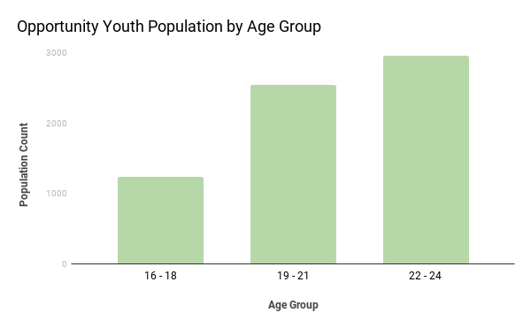
We decided to break the OY population into three age groups: 16-18yo, 19-21yo, 22-24yo. This was so we could make comparisons with the 2016 report as well as being able to capture the potentially unique circumstances of each group.
From this bar graph, we can see that the population of OY is highest for the 22-24 year olds and lowest for the 16-18 year olds. This might be a trend we expect to see, since 16-18 years are more likely to still be under the supervison of family members and/or adults and so have more accountability to be in school or working.
Further investigation into the living situations of OY 19 and older might shed light on the factors contributing to their school enrollment and employment status.
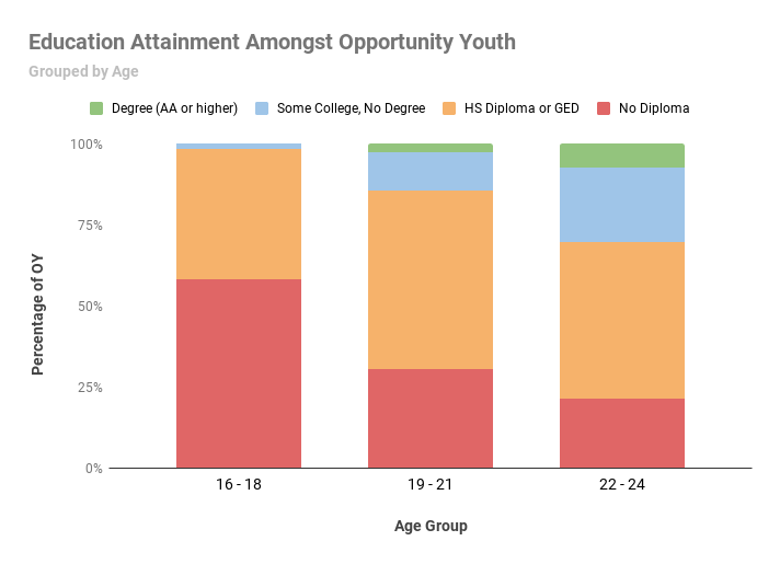
Since education is one of the definig factors of OY, it seems necessary to investigate the levels of education this population has attained, given that they are not currently in school.
Across all ages, 49% of Opportunity Youth had a high school diploma or a GED. We can see from the figure above that, when broken down by age group, we can see that 55% of 19-21yo and 48% of 22-24yo have achieved a high school diploma or GED whereas 58% of the 16-18yo have not attained a diploma. This is not too surprising given that people between 16-18 years old are 'school aged', so it is typical to see 16-18yo without a diploma. Further investigation into these circumstances is necessary.
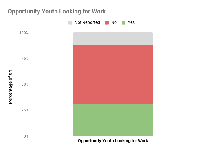
As employment is the second defining factor of Opportunity Youth, it is compelling to look into the motivations Opportunity Youth have toward seeking employment.
While 12% of the data was not reported, 56.7% of Opportunity Youth reported 'No' in the survey, in response to the category 'Looking for Work' (80% of which came from ages 19-24). This sparks the question "why are Opportunity Youths not looking for work if they are neither in school or working?".
Our analysis so far has highlighted the need for further investigation into the education and employment status' of the Opportunity Youth.
Variables such as motivation for seeking education or employment, living circumstances and accountability systems for each age group require further research to gain a deeper understanding of the characteristics defining Opportunity Youth.
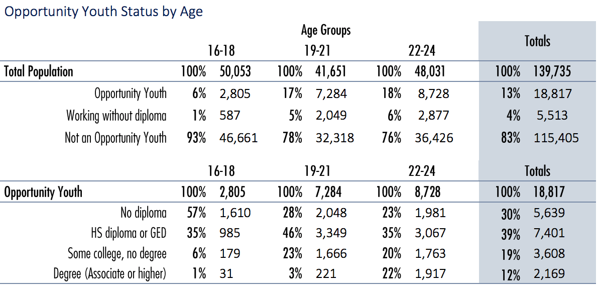
In Part 3 of this analysis, we present updates on the "Opportunity Youth Status by Age" table from the 2016 report "Opportunity Youth in the Road Map Project Region".
We also highlight the discrepancies that are present between the two data sets.
First, we take a look at the 2014 data, as reported in 2016.
As mentioned earlier, the specifics are unclear as to how the 2016 report defined the South King County region. We believe this had an effect on the total population size that was reported.
Further to this, the 2016 report did not include people who were 'working without a diploma' in the 'Non-Opportunity Youth' category. This conflicted with our definition of what constitutes an Opportunity Youth and so we chose to include 'working without a diploma' persons in our count for 'Non-Opportunity Youth' persons. You will see in our updated table that we have shared the number of people who are working without a diploma, however, these people were already counted in our 'Not an Opportunity Youth' count, so we did not add them to our total counts to avoid double counting them.
Firstly, the significant difference between the size of the population reported in 2016 versus the size of the population we have calculated can be attributed to how we defined South King County.
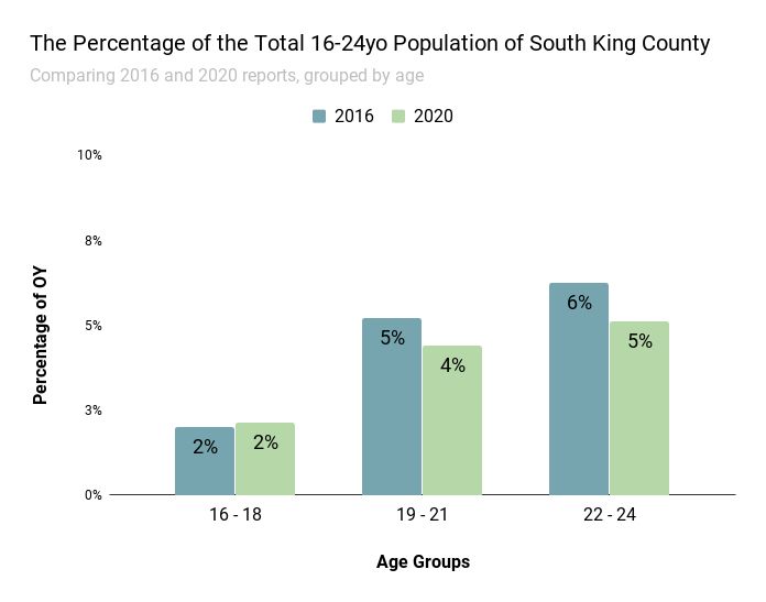
When comparing the tables, a similarity between the proprtion of the populations is evident. For example, in the 2016 report, 13% of the total (16-24yo) population was reported as Opportunity Youth. Similarily, we have found that 12% of the total (16-24yo) population was Opportunity Youth. This can be seen in the bar graph below where we also highlight the similarities in the proportions of OY by each age group across the two reporting years:
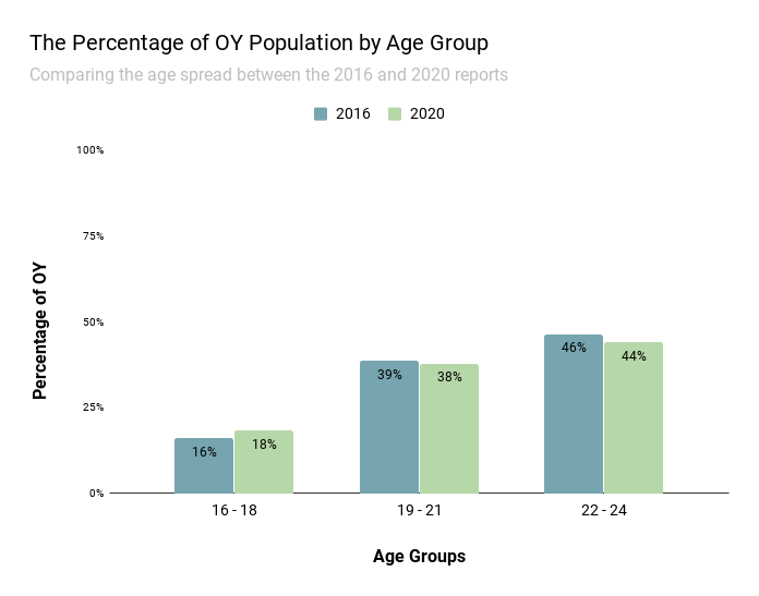
We can also see that the distribution of age groups is also fairly similar between the 2014 data and 2017 data. As was noted in part 2 of this analysis, there is an upward trend in the OY population by age; that is, the lowest portion of the population is the 16-18yo and the highest portion lies in the 22-24yo group. We see a similar trend in the 2014 data as can be seen here.
In part 3 of this analysis, we discussed the similarities between the 2016 findings and our own. We saw that while the sampling region of the two reports differed, resulting in a larger reported population for the 2016 report, the proportions of the OY population remained much the same between the 2014 and 2017 data.
In this section we were looking for a trend between the 2016 report and our current data.
Reviewing the data provided by the 2016 report and comparing it to the numbers generated by our analysis in 2 & 3 we were struck by what appeared to be a remarkable drop in the number of OY.
While there is a significant difference in the number of OY in the data collected, when the data is reframed to consider the makeup of the age groups by percentage rather than headcount, we see that there has not been a significant change in the overall makeup of the OY age groups.
This report set out to highlight areas for future investigation in order to gain a better understanding of the Opportunity Youth population. By diving deeper into the reasons for the levels of education that the Opportunity Youth attain, and the factors that motivate Opportunity Youth to seek employment, a better understanding of this population can be formed to drive future efforts of support.
