The goal of this project is to classify different species of birds as accurately as possible. There is a competition hosted on Kaggle that provides dataset for training and testing as well as the utility to measure accuracy.
The dataset provided consists of colored images of birds. The training set consists of over 38,000 images with 555 different types of birds, and the test set consists of 10,000 images. The true label of the test set is not provided.
The best tool for image classification tasks we know of is deep neural networks. More specifically, convolution neural networks (CNN) are particularly good at image classification due to the fact that pixels closed by are more correlated than pixels far apart. So the high level approach is to train a deep neural network with primarily convolution layers to classify birds.
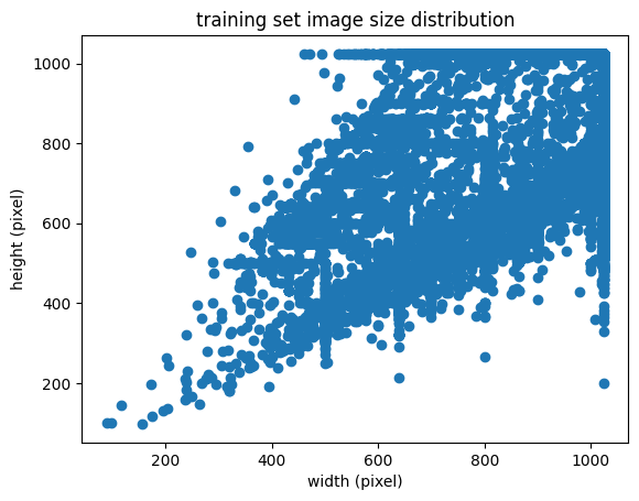
The data provided consists of colored images of birds that are not the same size. For consistency, the image is cropped to a fixed size before feeding into the neural network. The size of the image affects the training speed and accuracy. We found that larger image size provides more accurate classification but slows down the training and evaluation process. 128x128, 224x224, and 256x256 are tried during this project.
To provide more diverse data, several data augmentation techniques are used, including random horizontal flip, random crop, and color jittering. The data augmentation techniques that are not used due to limited time are random rotation and normalization.
Since the true labels of test data are hidden, we split 10% randomly off from the provided training set as a validation set. This allows us to better control the training process as we can evaluate the accuracy on validation set after each epoch to gain insight about the test accuracy.
There are many successful neural network architectures for image classifications. In most cases, they consist of many blocks, and each block consists of convolution layers, max pooling layers, and normalization layers. In the end, the output of the last block is flattened, and a fully connected layer is used to map it to the final classification result, a vector of size n, representing the score for each class.
In a fully trained network, layers before the final linear layers behave like feature extractors that progressively extract higher levels of features. Many of these features are independent of the classification task. This enables transfer learning, a technique of reusing part of weights of a trained network for different tasks. Transfer learning also has the benefit of providing better accuracy, as those weights could be trained from a much broader dataset than the task at hand. In general, weights from the previous layers of the existing network can be frozen so that their gradient won’t change during transfer learning. This could result in faster training time but worse accuracy. In this project, we did not freeze the weights. We initialized resnet and efficientnet using pretrained weights, reset their final fully connected layer and train them on this dataset to classify birds.
There are no particular technical reasons for choosing these architectures. We choose them because pretrained weights of these models are easily accessible.
===============================================================================================
Layer (type:depth-idx)                        Output Shape              Param #
===============================================================================================
EfficientNet                                  [32, 555]                 --
├─Conv2d: 1-1                                 [32, 48, 112, 112]        1,296
├─BatchNormAct2d: 1-2                         [32, 48, 112, 112]        96
│    └─Identity: 2-1                          [32, 48, 112, 112]        --
│    └─SiLU: 2-2                              [32, 48, 112, 112]        --
├─Sequential: 1-3                             [32, 512, 7, 7]           --
│    └─Sequential: 2-3                        [32, 24, 112, 112]        --
│    │    └─DepthwiseSeparableConv: 3-1       [32, 24, 112, 112]        2,940
│    │    └─DepthwiseSeparableConv: 3-2       [32, 24, 112, 112]        1,206
│    │    └─DepthwiseSeparableConv: 3-3       [32, 24, 112, 112]        1,206
│    └─Sequential: 2-4                        [32, 40, 56, 56]          --
│    │    └─InvertedResidual: 3-4             [32, 40, 56, 56]          13,046
│    │    └─InvertedResidual: 3-5             [32, 40, 56, 56]          27,450
│    │    └─InvertedResidual: 3-6             [32, 40, 56, 56]          27,450
│    │    └─InvertedResidual: 3-7             [32, 40, 56, 56]          27,450
│    │    └─InvertedResidual: 3-8             [32, 40, 56, 56]          27,450
│    └─Sequential: 2-5                        [32, 64, 28, 28]          --
│    │    └─InvertedResidual: 3-9             [32, 64, 28, 28]          37,098
│    │    └─InvertedResidual: 3-10            [32, 64, 28, 28]          73,104
│    │    └─InvertedResidual: 3-11            [32, 64, 28, 28]          73,104
│    │    └─InvertedResidual: 3-12            [32, 64, 28, 28]          73,104
│    │    └─InvertedResidual: 3-13            [32, 64, 28, 28]          73,104
│    └─Sequential: 2-6                        [32, 128, 14, 14]         --
│    │    └─InvertedResidual: 3-14            [32, 128, 14, 14]         91,664
│    │    └─InvertedResidual: 3-15            [32, 128, 14, 14]         256,800
│    │    └─InvertedResidual: 3-16            [32, 128, 14, 14]         256,800
│    │    └─InvertedResidual: 3-17            [32, 128, 14, 14]         256,800
│    │    └─InvertedResidual: 3-18            [32, 128, 14, 14]         256,800
│    │    └─InvertedResidual: 3-19            [32, 128, 14, 14]         256,800
│    │    └─InvertedResidual: 3-20            [32, 128, 14, 14]         256,800
│    └─Sequential: 2-7                        [32, 176, 14, 14]         --
│    │    └─InvertedResidual: 3-21            [32, 176, 14, 14]         306,048
│    │    └─InvertedResidual: 3-22            [32, 176, 14, 14]         496,716
│    │    └─InvertedResidual: 3-23            [32, 176, 14, 14]         496,716
│    │    └─InvertedResidual: 3-24            [32, 176, 14, 14]         496,716
│    │    └─InvertedResidual: 3-25            [32, 176, 14, 14]         496,716
│    │    └─InvertedResidual: 3-26            [32, 176, 14, 14]         496,716
│    │    └─InvertedResidual: 3-27            [32, 176, 14, 14]         496,716
│    └─Sequential: 2-8                        [32, 304, 7, 7]           --
│    │    └─InvertedResidual: 3-28            [32, 304, 7, 7]           632,140
│    │    └─InvertedResidual: 3-29            [32, 304, 7, 7]           1,441,644
│    │    └─InvertedResidual: 3-30            [32, 304, 7, 7]           1,441,644
│    │    └─InvertedResidual: 3-31            [32, 304, 7, 7]           1,441,644
│    │    └─InvertedResidual: 3-32            [32, 304, 7, 7]           1,441,644
│    │    └─InvertedResidual: 3-33            [32, 304, 7, 7]           1,441,644
│    │    └─InvertedResidual: 3-34            [32, 304, 7, 7]           1,441,644
│    │    └─InvertedResidual: 3-35            [32, 304, 7, 7]           1,441,644
│    │    └─InvertedResidual: 3-36            [32, 304, 7, 7]           1,441,644
│    └─Sequential: 2-9                        [32, 512, 7, 7]           --
│    │    └─InvertedResidual: 3-37            [32, 512, 7, 7]           1,792,268
│    │    └─InvertedResidual: 3-38            [32, 512, 7, 7]           3,976,320
│    │    └─InvertedResidual: 3-39            [32, 512, 7, 7]           3,976,320
├─Conv2d: 1-4                                 [32, 2048, 7, 7]          1,048,576
├─BatchNormAct2d: 1-5                         [32, 2048, 7, 7]          4,096
│    └─Identity: 2-10                         [32, 2048, 7, 7]          --
│    └─SiLU: 2-11                             [32, 2048, 7, 7]          --
├─SelectAdaptivePool2d: 1-6                   [32, 2048]                --
│    └─AdaptiveAvgPool2d: 2-12                [32, 2048, 1, 1]          --
│    └─Flatten: 2-13                          [32, 2048]                --
├─Linear: 1-7                                 [32, 555]                 1,137,195
===============================================================================================
Total params: 29,477,979
Trainable params: 29,477,979
Non-trainable params: 0
Total mult-adds (G): 75.38
===============================================================================================
Input size (MB): 19.27
Forward/backward pass size (MB): 5995.66
Params size (MB): 117.22
Estimated Total Size (MB): 6132.15
===============================================================================================
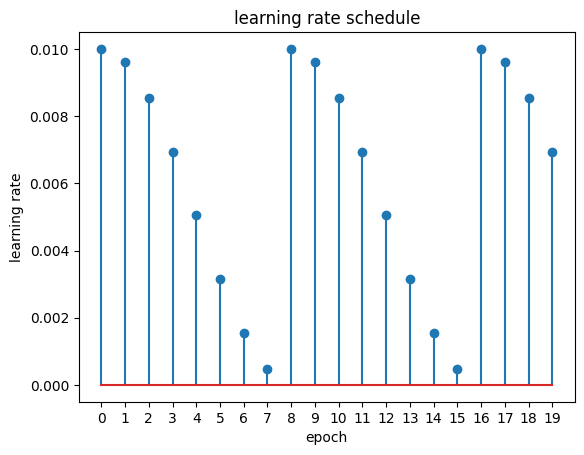
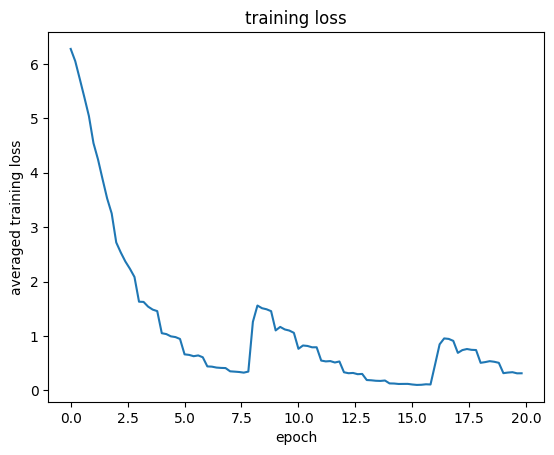
To train the model, we used the stochastic gradient descent optimizer (SDG) from pytorch. Based on previous experiences with neural networks, we found that a LR of 0.01, momentum of 0.9 and weight decay of 0.001 a good starting point. However, the model begin to plateau (i.e., the losses did not decrease across epochs) as we reached 14 epochs. To improve the model, we used the cosine annealing learning rate scheduler to vary learning rate across the training process. This scheduler also reset itself after certain epochs This enables us to train the model longer before it plateaus and therefore getting a better accuracy.
As a baseline, we used the provided example to train a resnet18 model with 128x128 input size for 5 epoch. This resulted in a final training loss of around 1.0 and a test accuracy of 54.6%. We then tried increase the input size to 256x256 and got a test accuracy of 67.45%. In the third attempt, we trained efficientnet_b5 model with 256x256 input for 14 epochs. To prevent out-of-memory error, we also lowered the batch size to 32 from 128. This took a long time, and we got 72.5% test accuracy. Finally, we implemented validation set, improved data augmentation, and cosine annealing learning rate, and changed the image input size to 224x224 as mentioned above. We got 76.7% test accuracy at 8 epoch (training loss 0.3) and 80.45% test accuracy at 16 epoch (training loss 0.1). We believe we can improve it slightly more at 24 epoch where the learning rate reaches the minimum value in the third cycle if we have more time.
Training large models takes a lot of memory and a long time. A problem we encountered a lot is running out of GPU memory and the notebook sessions from Kaggle or Colab shutsdown/crashes as we are training. We ended up training efficientnet locally on a macbook pro with 32GB unified memory (as most available GPUs only have 16GB memory) using pytorch's MPS backend acceleration. We also reduces the batch size to 32 from 128, as we found that this substantially reduces memory needed.
Based on the experiments, improved data augmentation, and cosine annealing learning rate definitely helps with the performance of the model. If we have more time, we would like to experiment with other data augmentation approaches, further improve the training process (such as using different optimizers), and incorporate other techniques such as dropout layer. We might also explore more sophasticated techniques such model ensembles, which combines multiple weaker models to create a stronger model.
SGDR: Stochastic Gradient Descent with Warm Restarts
Deep Residual Learning for Image Recognition
EfficientNet: Rethinking Model Scaling for Convolutional Neural Networks


