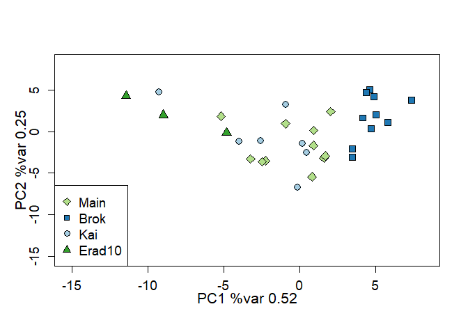
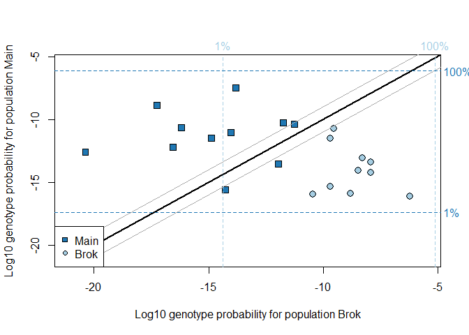
Changed to using Rcpp for internal saddlepoint calculations (Version 0.1.0 used all R code).
Also changed to use leave-one-out mode by default.
Other changes are cosmetic and/or internal.
geneplot is an R package for genetic assignment and analysis of
population structure. It can be used with microsatellite or SNP data.
The algorithms are related to the GENECLASS2 software package.
geneplot provides visualizations of the population structure and
assignment results.
geneplot can be used to compare the genetic patterns of different
populations, to assess the level of genetic connectedness or separation
among them. It also performs genetic assignment, comparing individuals
to populations to determine the source population of each individual
i.e. the population that the individual originated from.
You can install the released version of geneplot from GitHub with:
# Install geneplot from GitHub
remotes::install_github("lfmcmillan/geneplot")

# Load the geneplot package
library(geneplot)Read the short introductory vignette to get you started with
geneplot, and have a look at the simple, reproducible examples of
the geneplot function.
# Read the short vignette
vignette("introduction-to-geneplot")
# Reproduce a simple example
example(geneplot)
If you want to use Genepop-format data in geneplot, there’s a simple
extra step to import it, as described in the Genepop format vignette:
vignette("importing-genepop-format")The following code creates a dataset in the format suitable for GenePlot, which has columns for individual IDs and population/sample labels, and then two columns for each locus, named in the pattern Loc1.a1, Loc1.a2, Loc2.a1, Loc2.a2, etc. The ‘pop’ column containing the population/sample labels must be strings rather than factors.
 ratLocnames <- c("D10Rat20","D11Mgh5","D15Rat77","D16Rat81","D18Rat96","D19Mit2","D20Rat46","D2Rat234","D5Rat83","D7Rat13")
 ratData <- rbind(
 c("Ki001","Kai",96,128,246,280,234,250,155,165,226,232,219,231,149,149,101,127,174,176,164,182),
 c("Ki002","Kai",122,126,246,276,238,238,155,165,226,232,223,231,187,187,107,121,174,174,164,164),
 c("Ki003","Kai",122,122,276,280,234,234,157,165,244,244,231,231,187,187,107,107,174,174,164,182),
 c("Ki004","Kai",130,130,276,280,238,238,157,165,0,0,223,231,187,187,101,111,168,176,184,184),
 c("Ki009","Kai",122,122,276,276,234,236,165,165,240,244,229,231,187,187,89,101,174,176,164,164),
 c("Ki010","Kai",122,122,278,280,236,236,155,165,236,244,219,231,185,187,101,101,168,174,164,164),
 c("Ki011","Kai",120,128,280,282,236,238,155,165,226,236,223,231,149,149,99,101,174,174,164,164),
 c("Bi01","Brok",96,126,280,280,236,250,165,165,232,246,231,231,185,187,89,89,170,176,154,164),
 c("Bi02","Brok",96,126,280,280,250,262,155,155,232,232,231,233,149,185,127,127,174,174,164,166),
 c("Bi03","Brok",96,126,280,280,258,262,165,165,232,232,231,231,185,187,89,127,174,174,164,164),
 c("Bi04","Brok",96,126,280,280,238,262,155,155,232,232,231,233,149,185,127,127,174,174,164,164),
 c("Bi05","Brok",96,122,280,280,250,258,155,155,226,244,231,231,187,187,107,127,174,176,164,164),
 c("Bi06","Brok",96,96,280,280,238,262,155,155,232,232,231,231,187,187,123,127,174,174,164,164),
 c("Bi11","Brok",96,96,278,280,234,250,165,165,226,240,231,231,149,187,89,99,170,170,154,164),
 c("Bi12","Brok",96,96,276,280,234,250,165,165,240,240,231,231,187,187,89,99,170,174,154,164),
 c("Bi13","Brok",96,126,276,276,246,250,165,165,226,244,231,231,149,187,99,99,174,174,164,164),
 c("Bi14","Brok",96,126,276,276,262,262,155,165,226,244,231,231,149,187,89,107,170,174,154,164),
 c("Ki092","Main",122,126,280,282,234,238,165,165,236,240,231,231,149,187,95,95,0,0,164,164),
 c("Ki093","Main",122,126,282,282,238,238,165,165,236,240,231,231,149,187,95,107,166,174,164,182),
 c("Ki094","Main",122,126,280,282,238,238,165,165,226,240,231,231,173,187,95,127,174,176,154,182),
 c("Ki095","Main",120,126,280,280,234,236,155,165,244,246,231,231,161,187,123,127,174,174,154,154),
 c("Ki097","Main",122,126,280,280,236,236,163,165,236,242,219,231,149,161,107,115,166,174,164,166),
 c("Ki098","Main",96,122,276,280,236,238,155,165,242,244,233,233,149,187,99,107,174,174,164,164),
 c("Ki100","Main",122,122,280,280,234,234,155,165,236,236,219,235,0,0,107,107,174,176,164,164),
 c("Ki101","Main",122,126,276,280,234,238,155,155,236,244,229,231,0,0,101,101,0,0,164,182),
 c("Ki102","Main",122,126,0,0,0,0,155,163,0,0,229,231,0,0,107,107,0,0,0,0),
 c("Ki103","Main",122,122,280,280,234,236,163,165,0,0,231,233,0,0,99,107,0,0,164,184),
 c("Ki104","Main",96,126,276,280,236,238,157,165,230,246,231,231,149,187,107,107,0,0,164,164),
 c("Ki105","Main",122,126,276,280,238,250,157,165,226,244,217,231,0,0,111,121,174,174,164,164),
 c("R01","Erad10",128,128,280,288,234,244,155,165,242,244,231,231,149,149,107,107,174,174,164,166),
 c("R02","Erad10",128,130,276,288,238,244,155,155,228,244,223,231,149,149,101,111,174,174,164,166),
 c("R03","Erad10",128,130,276,288,238,244,155,155,244,244,223,231,149,187,107,111,174,176,164,166))
 ratData <- as.data.frame(ratData, stringsAsFactors=FALSE)
 names(ratData) <- c("id","pop","D10Rat20.a1","D10Rat20.a2","D11Mgh5.a1","D11Mgh5.a2",
                     "D15Rat77.a1","D15Rat77.a2","D16Rat81.a1","D16Rat81.a2",
                     "D18Rat96.a1","D18Rat96.a2","D19Mit2.a1","D19Mit2.a2",
                     "D20Rat46.a1","D20Rat46.a2","D2Rat234.a1","D2Rat234.a2",
                     "D5Rat83.a1","D5Rat83.a2","D7Rat13.a1","D7Rat13.a2")
The populations/samples in this dataset are Kai, Main, Brok and Erad10.
This is a basic example of running GenePlot using the dataset created above:
## Running geneplot on two populations, Brok and Main:
geneplot(ratData, c("Brok","Main"), locnames=ratLocnames)
#> Removing  1 individuals with number of loci <  6
#> id pop status nloc Brok Main Brok.raw Main.raw
#> 8 Bi01 Brok complete 10 -10.463155 -15.962398 -10.463155 -15.962398
#> 9 Bi02 Brok complete 10 -8.796691 -15.919349 -8.796691 -15.919349
#> 10 Bi03 Brok complete 10 -6.204291 -16.107949 -6.204291 -16.107949
#> 11 Bi04 Brok complete 10 -7.931389 -14.214627 -7.931389 -14.214627
#> 12 Bi05 Brok complete 10 -9.527735 -10.745273 -9.527735 -10.745273
#> 13 Bi06 Brok complete 10 -7.924364 -13.380205 -7.924364 -13.380205
#> 14 Bi11 Brok complete 10 -9.692142 -15.363519 -9.692142 -15.363519
#> 15 Bi12 Brok complete 10 -8.289629 -13.090892 -8.289629 -13.090892
#> 16 Bi13 Brok complete 10 -9.679080 -11.492340 -9.679080 -11.492340
#> 17 Bi14 Brok complete 10 -8.466085 -14.086351 -8.466085 -14.086351
#> 19 Ki093 Main complete 10 -17.260941 -8.896318 -17.260941 -8.896318
#> 20 Ki094 Main complete 10 -14.874779 -11.501816 -14.874779 -11.501816
#> 21 Ki095 Main complete 10 -11.957049 -13.542455 -11.957049 -13.542455
#> 22 Ki097 Main complete 10 -20.374850 -12.581399 -20.374850 -12.581399
#> 23 Ki098 Main complete 10 -11.244062 -10.364003 -11.244062 -10.364003
#> 18 Ki092 Main impute 9 -13.825510 -7.471357 -12.899253 -7.265848
#> 24 Ki100 Main impute 9 -16.186408 -10.644076 -15.175800 -9.737994
#> 25 Ki101 Main impute 8 -16.553048 -12.197220 -14.508189 -10.235903
#> 27 Ki103 Main impute 7 -14.016101 -11.028628 -10.510145 -7.412479
#> 28 Ki104 Main impute 9 -11.743141 -10.249605 -10.885405 -9.708348
#> 29 Ki105 Main impute 9 -14.257180 -15.602244 -13.280560 -13.833248
## Running geneplot on all the populations in the dataset, and capturing the output in the results object:
results <- geneplot(ratData, unique(ratData$pop), locnames=ratLocnames)
#> Removing 1 individuals with number of loci < 6
The main function in the geneplot package is geneplot. This runs the
GenePlot calculations and also plots the graphs.
You can alternatively run the calculations using calc_logprob and then
produce the plots using plot_logprob. The output of calc_logprob is
the same as the output of GenePlot, and can then be passed into
plot_logprob. This can be useful if you want to run the calculations
just once, and then rerun the plot function to test different colour
combinations and display options on the same calculated results.
## Running geneplot on two populations, Brok and Main:
results <- calc_logprob(ratData, c("Brok","Main"), locnames=ratLocnames)
#> Removing  1 individuals with number of loci <  6

## Running geneplot on all the populations in the dataset:
plot_logprob(results)The vignette ‘importing-genepop-format’ describes how to import data
from a Genepop-format file into the form required by geneplot.
Here is a quick example of code that would import a file in Genepop
format, using 3 digits per allele and specifying the population names
using the pop_names input. After importing the Genepop-format data, the
data and the names of the loci must be passed separately into the
geneplot function, and the user also has to specify which populations
to use.
genepopData <- read_genepop_format(file="C:/Users/me/Documents/myfile.gen", digits_per_allele=3, pop_names=c("PopA","PopB","PopC"))
dat <- genepopData$popData
locnames <- genepopData$locnames

geneplot(dat=dat,refpopnames=c("PopA","PopB"),locnames=locnames)citation("geneplot")
#>
#> To cite geneplot in publications use:
#>
#> McMillan and Fewster (2017). Visualizations for genetic assignment
#> analyses using the saddlepoint approximation method. Biometrics,
#> 73(3), 1029--1041. URL
#> https://onlinelibrary.wiley.com/doi/abs/10.1111/biom.12667.
#>
#> A BibTeX entry for LaTeX users is
#>
#> @Article{,
#> title = {Visualizations for genetic assignment analyses using the saddlepoint approximation method},
#> author = {{McMillan} and L. F. and {Fewster} and R. M.},
#> journal = {Biometrics},
#> year = {2017},
#> volume = {73},
#> number = {3},
#> pages = {1029--1041},
#> doi = {10.1111/biom.12667},
#> url = {https://onlinelibrary.wiley.com/doi/abs/10.1111/biom.12667},
#> abstract = {We propose a method for visualizing genetic assignment data by characterizing the distribution of genetic profiles for each candidate source population. This method enhances the assignment method of Rannala and Mountain (1997) by calculating appropriate graph positions for individuals for which some genetic data are missing. An individual with missing data is positioned in the distributions of genetic profiles for a population according to its estimated quantile based on its available data. The quantiles of the genetic profile distribution for each population are calculated by approximating the cumulative distribution function (CDF) using the saddlepoint method, and then inverting the CDF to get the quantile function. The saddlepoint method also provides a way to visualize assignment results calculated using the leave-one-out procedure. This new method offers an advance upon assignment software such as geneclass2, which provides no visualization method, and is biologically more interpretable than the bar charts provided by the software structure. We show results from simulated data and apply the methods to microsatellite genotype data from ship rats (Rattus rattus) captured on the Great Barrier Island archipelago, New Zealand. The visualization method makes it straightforward to detect features of population structure and to judge the discriminative power of the genetic data for assigning individuals to source populations.},
#> }

