The goals / steps of this project are the following:
- Compute the camera calibration matrix and distortion coefficients given a set of chessboard images.
- Apply a distortion correction to raw images.
- Use color transforms, gradients, etc., to create a thresholded binary image.
- Apply a perspective transform to rectify binary image ("birds-eye view").
- Detect lane pixels and fit to find the lane boundary.
- Determine the curvature of the lane and vehicle position with respect to center.
- Warp the detected lane boundaries back onto the original image.
- Output visual display of the lane boundaries and numerical estimation of lane curvature and vehicle position.
The code for the camera calibration can be excuted by running the following:
python calibrate.py
It calculates the camera matrix and distortion coefficients and stores them in the cal.pckl file, which is later used for camera calibration.
I start by preparing "object points", which will be the (x, y, z) coordinates of the chessboard corners in the world. Here I am assuming the chessboard is fixed on the (x, y) plane at z=0, such that the object points are the same for each calibration image. Thus, objp is just a replicated array of coordinates, and objpoints will be appended with a copy of it every time I successfully detect all chessboard corners in a test image. imgpoints will be appended with the (x, y) pixel position of each of the corners in the image plane with each successful chessboard detection.
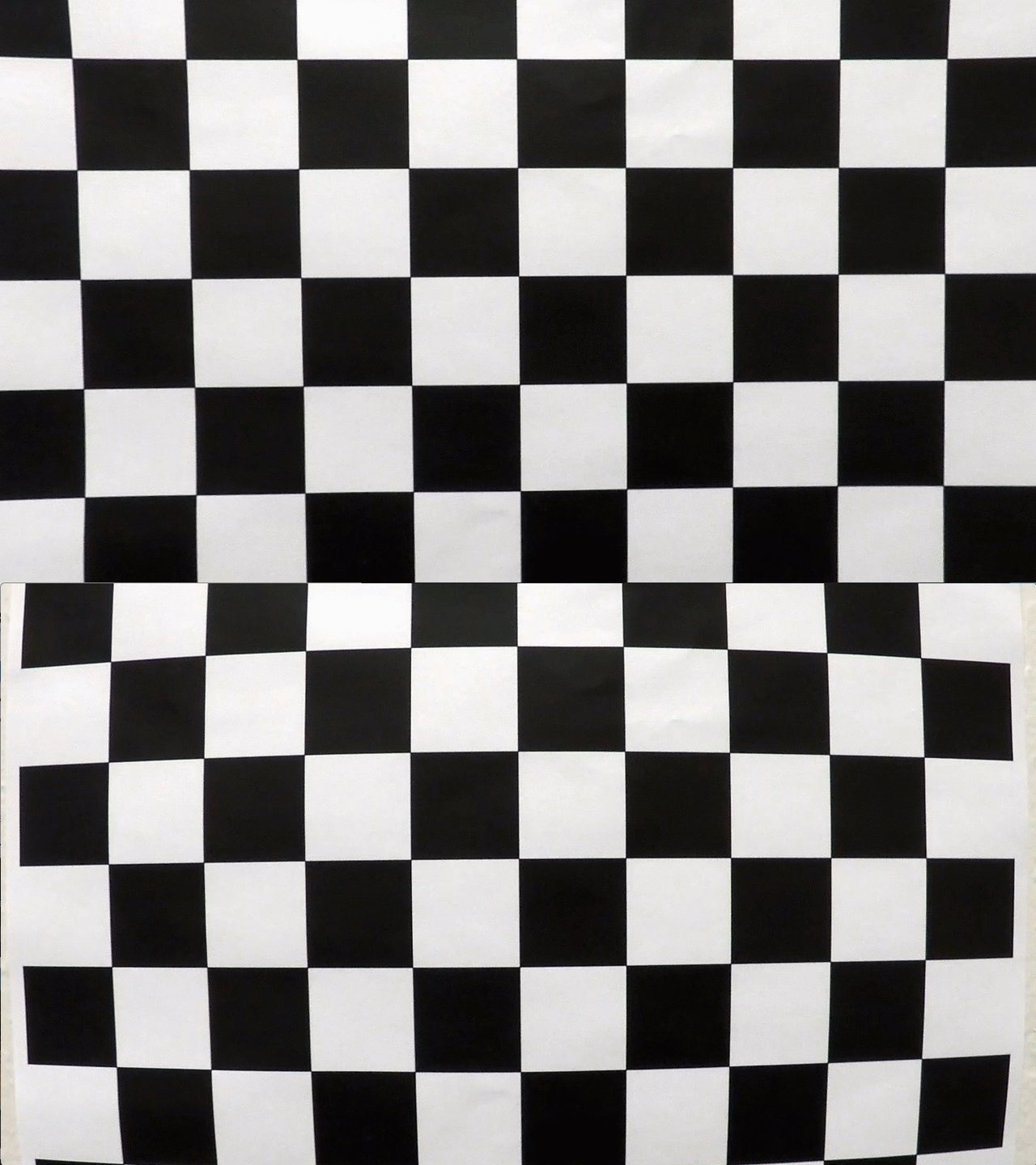
I then used the output objpoints and imgpoints to compute the camera calibration and distortion coefficients using the cv2.calibrateCamera() function. I applied this distortion correction to the test image using the cv2.undistort() function and obtained this result:
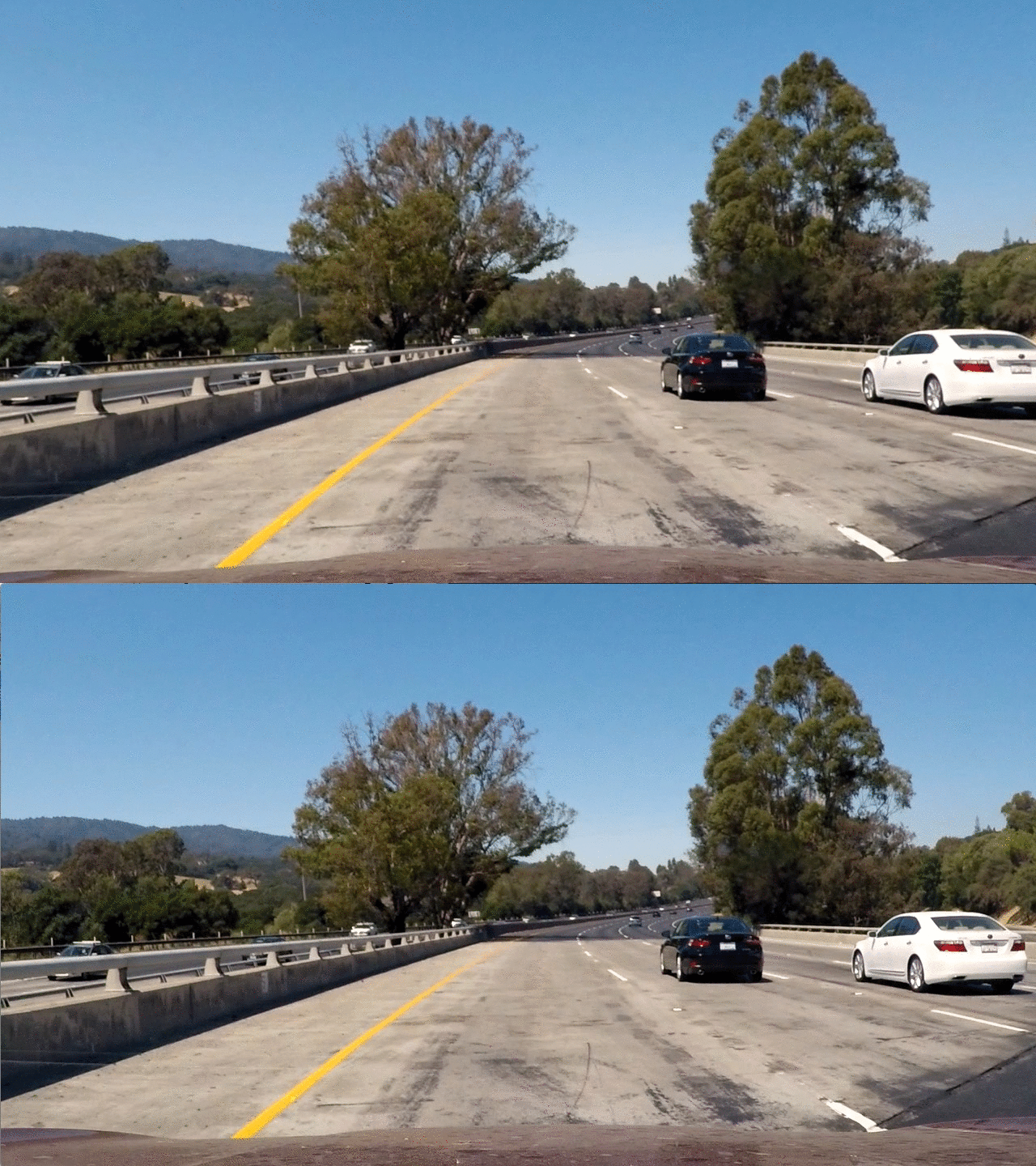
Here an example of a distortion-corrected image of real driving data is given as a gif to show the difference between the orignal and the distortion-corrected image:
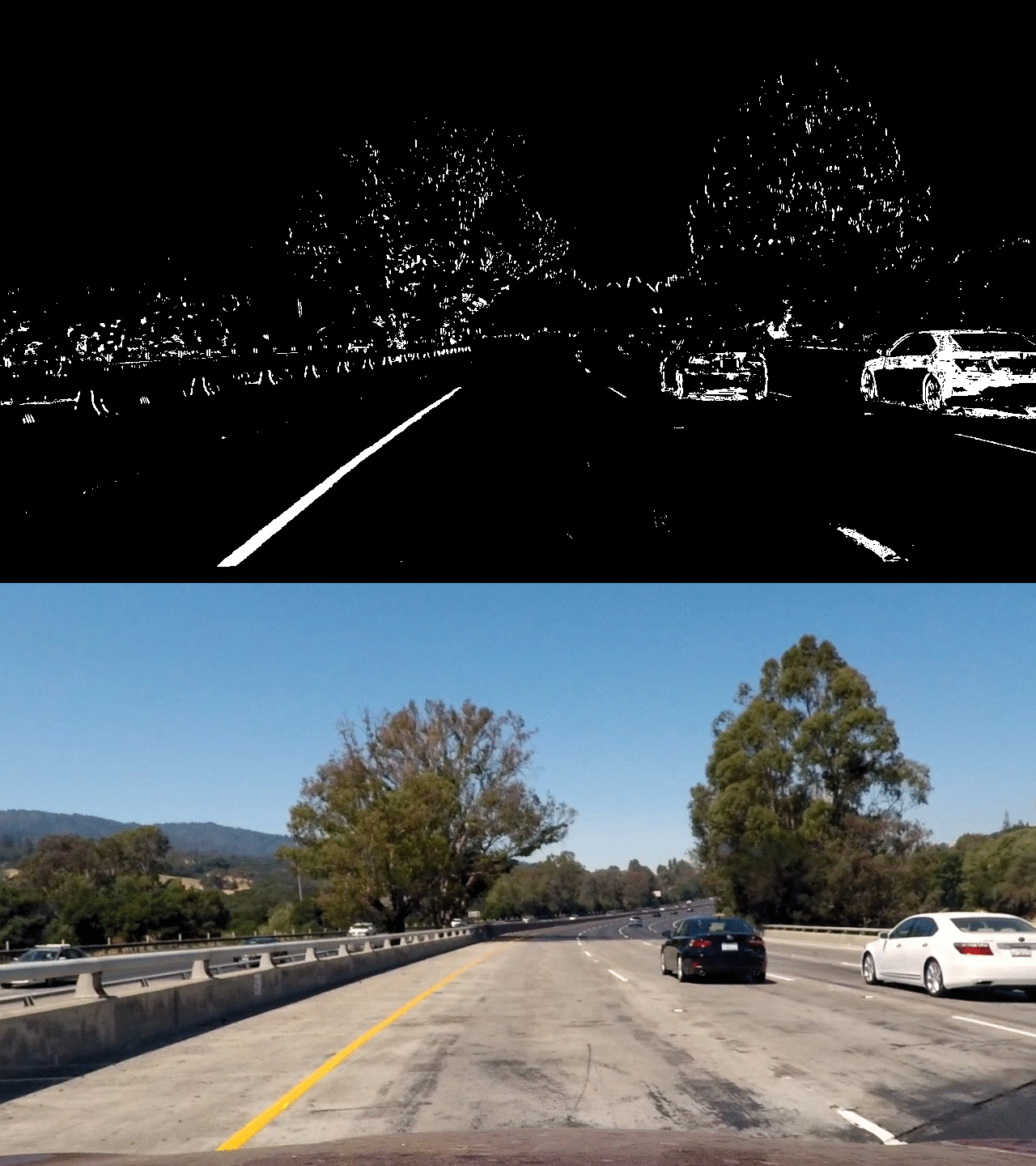
I used a combination of color and gradient thresholds to generate a binary image (thresholding steps at lines #11 through #96 in pipeline.py). Here's an example of my output for this step:
The shwon image is the result of a combination of:
- thresholding on the s-channel of HLS color space,
- maginitude,
- x/y-sobel,
- and direction of gradients.
The code for my perspective transform includes a function called warpPerspective(img), which appears in lines #99 through #116 in the file pipeline.py. The function takes as inputs an image img and uses hardcoded source and destination points derived from the two provided test images with straight road lines.
This resulted in the following source and destination points:
| Source | Destination |
|---|---|
| 705, 460 | 880, 0 |
| 1035, 670 | 880, 720 |
| 286, 670 | 400, 720 |
| 582, 460 | 400, 0 |
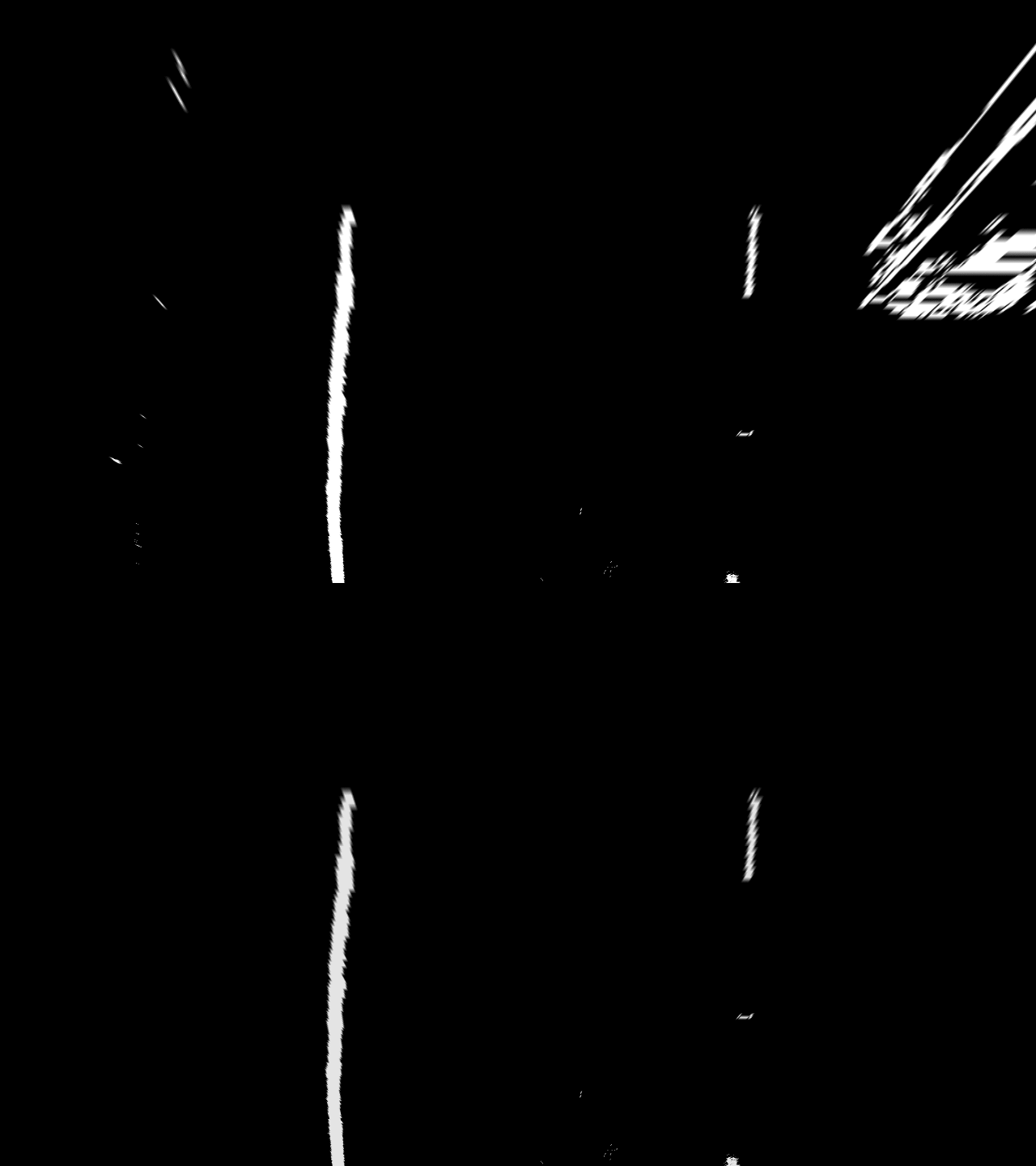
This yields the following perspective transformed image, before and after masking of artifacts on the left and right side:
For identifying lane-line pixels the provided code of the udacity class was used. To initially find the lines, the lower quarter of the images was scanned with a sliding window approach and the histogram was calculated for each row in the find_lanes(img) function in line #118. The two highest values of the left and right side of the histogram were choosen as inital points for the further finding of lane-line pixels. Afterwards, the image was horizontally separated in 9 parts. Outgoing from the inital points of the histogram the lane-line centers were calculated by finding the maximum points in the next part of the image with a margin of +/-25px from the last found center points. If at least 250 points were in the searched area, the found points were added to all lane-line pixels belonging to the left or right lane.
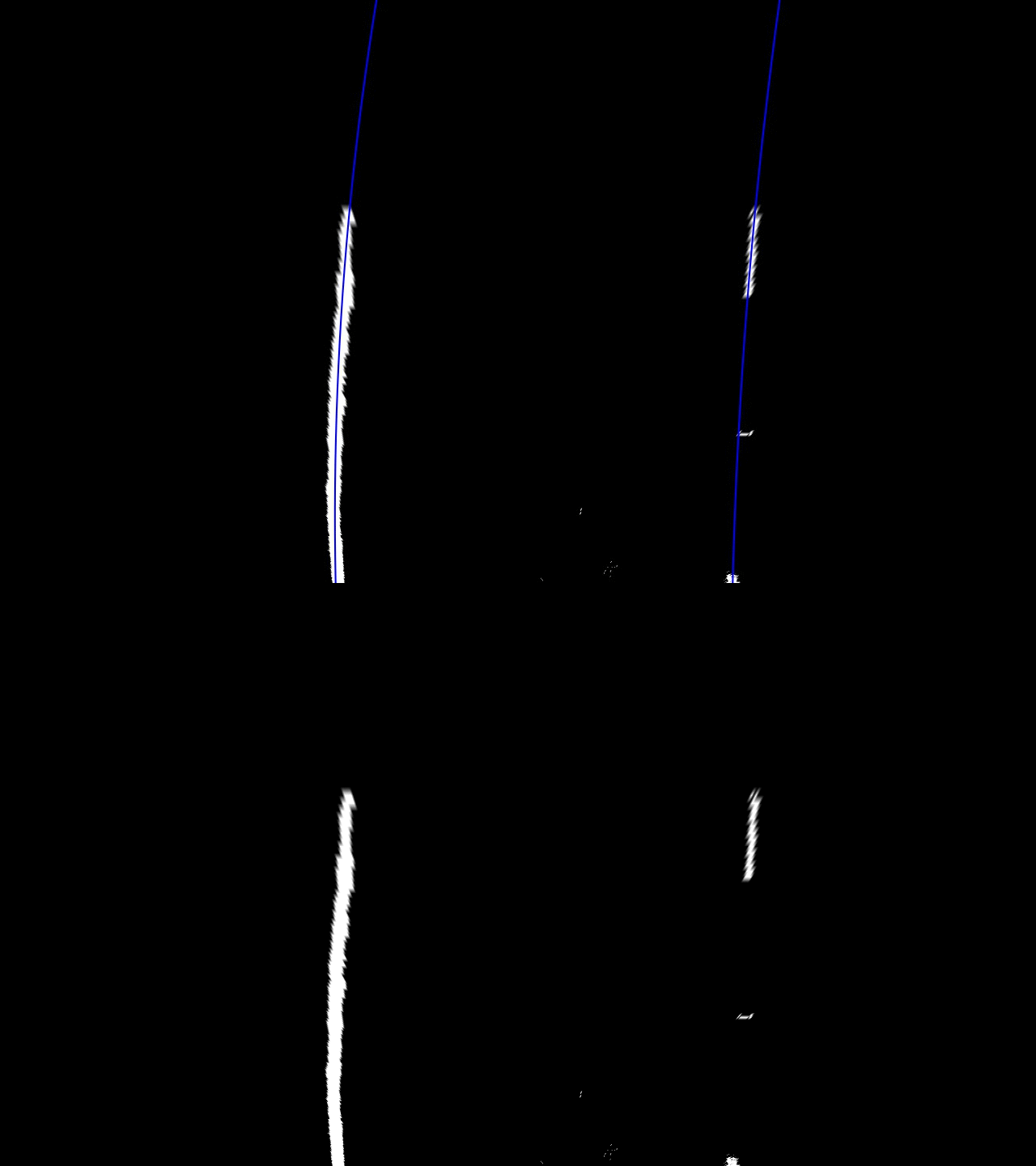
In the end, np.polyfit(x, y, 2) was used to fit a second order polynomial to these points. The following image shows the resulting polynomials:
If the lane lines were detected by find_lanes(img), the function fast_find_lanes(img) (line #195) was used instead. It directly adds all points with a margin of +/-25 around the fitted polynomials of the frame before the current.
The radius of curvature was calculated in the curvature(img, left_lane_inds, right_lane_inds) function (line #222), by using the provided function of the udacity class. The conversion factor in x-direction for pixel to metre was changed to 3.7m/480px, because the distance between lines changed in pixel space in the perspective transformation (400 left, 880 right). The factor for the y-direction was kept the same (30m/720px).
The lane position was calculated in the offset(undist, left_fit, right_fit) function (line #253). The left and right polynomaials were used to calculate the left and right lane position at the bottom of the image (lowest y-pixel position). Afterwards, the difference between the image center (car center) and the middle between both lines was calculated to provide the offset of the car from the center of the road.
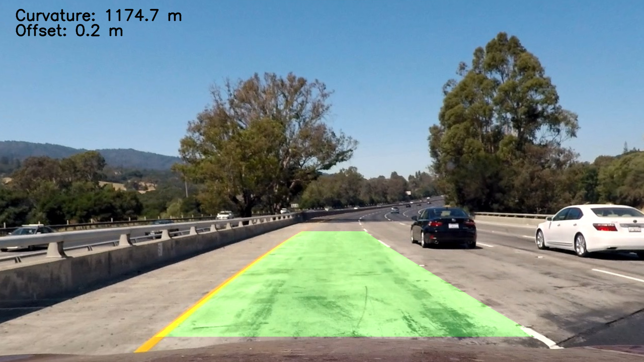
The final visualization was implemented in the draw(...) function in line #276. The inverse perspective transform is used to transform the area of between the fitted polynomials back on the undistorted frame. Further, the mean curvature of the left and right polynomials and the car lane offset are drawn on the upper left of the frame. The final visualization is shown below:
My pipeline for video handling cales the function run_image(img), which incorporates the whole single image pipeline discribed above, and writes the resulting image to the outputvideo.
Simple averageing of the last 5 measured polynomial coeffients is used to increase robustness and handle gaps of missed detections in some frames. The curvature calculation was averaged over the last 10 measurements.
Here's a link to my final video result. It performs well over the whole video sequence, of the project video.
Eventough the discribed pipeline performs well on the project video it has a lot of weaknesses:
-
Features: Gradients are combined with the
s-channelof HSV space to detect possible lane-line pixels. The problem with this is, that gradients from brighter to darker areas in the lane not belonging to the actual lines can distract or confuse the algorithm. Color features could be included to only detect white/yellow pixels. Therefore, thecombined_thresh(img)function in line #87 should be changed to combine thes-channelof the HSV space with the gradient binary images with anlogical andnot as done in this implementation with anlogical or. This should be evaluated in my future work. Furthermore, other features could be found e.g. based on pixel segmentation of an Autoencoder-Decoder Network. -
Sanity checks: The current implementation does not use sanity checks to evaluate, if the detected line make sense. Different logical rules could be used for checking, like parallelismn of polynomials, curvarture or distance of the lane-lines discribed in the class. Furthermore
Kalman-filteringor such could be used to increase robustness of the measured polynomial coefficents. -
Lane finding: The currently used algorithm to identify lane-lane pixels may fail to identify the correct lane pixels due to false positives in the binary image. This correlated with the used features and may be solved with better sanity checks. The lane-line pixsel identification can be made more robust by using e.g a
RANSACalgotithm. -
Strong lane curvature: The algorthim as is will fail on strong lane curvature due to a simple masking of the perspective transformed image. Furthermore, a relatively small
margin(#143, #222) of changes of the 9 bins of the image for lane-line pixel identifying is used to reduce the pissiblity of false positives in the project video, but will fail in some situations. Increasing the margin and not masking may help, but on the other hand it increases the number of false posivtive points for the polynomial fitting. In combination with the discribed improvements above, this problem may be solved.
