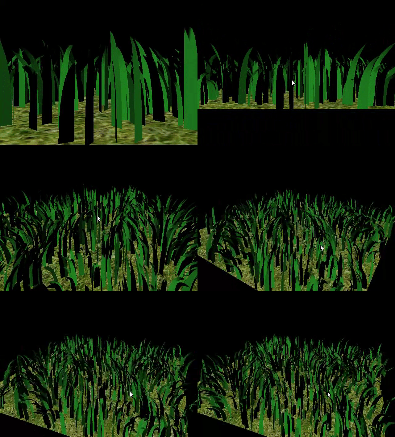
University of Pennsylvania, CIS 565: GPU Programming and Architecture, Project 6
- Liam Dugan -- Fall 2018
- Tested on: Windows 10, Intel(R) Xeon(R) CPU E5-2687W v3 @ 3.10GHz 32GB, TITAN V 28.4GB (Lab Computer)
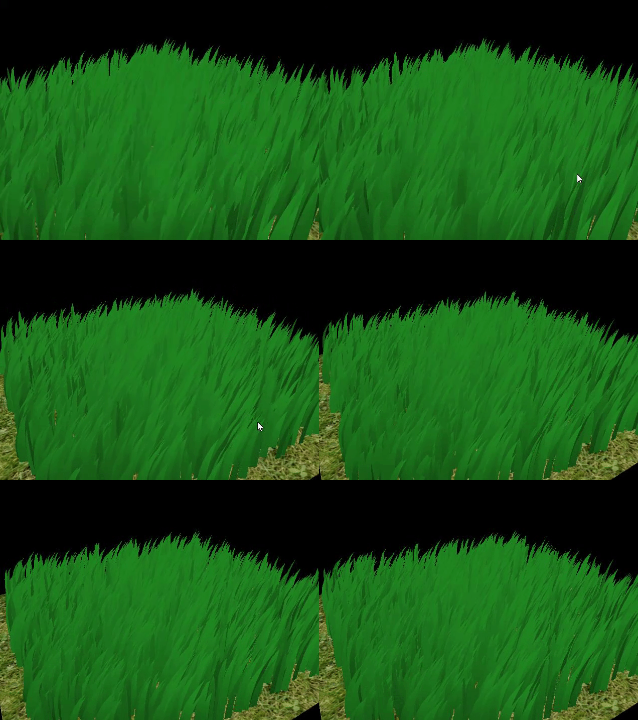
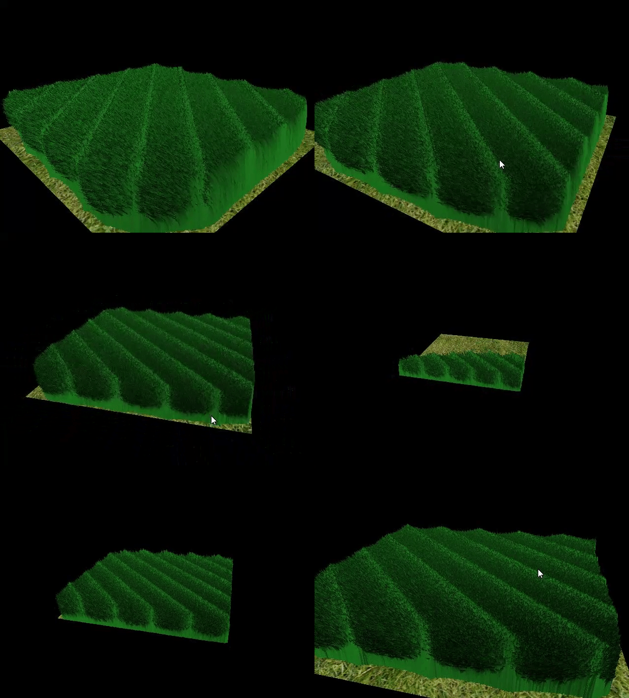
This project is an implementation of the paper, Responsive Real-Time Grass Rendering for General 3D Scenes.
It involves two different rendering passes. First there's a compute pass which calculates the forces exerted on the blades and decides whether or not the given blade should be culled, then the second render pass tessellates the culled grass blades to different levels of detail based on the bezier curve points' distance from the camera and renders them with simple Lambertian shading to get the final blade output.
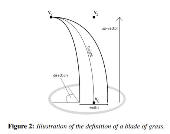
Grass blades are represented as Bezier curves while performing physics calculations and culling operations. Each Bezier curve has three control points.
v0: the position of the grass blade on the geomtryv1: a Bezier curve guide that is always "above"v0with respect to the grass blade's up vector (explained soon)v2: a physical guide for which we simulate forces on
We also store per-blade characteristics that will help us simulate and tessellate our grass blades correctly.
up: the blade's up vector, which corresponds to the normal of the geometry that the grass blade resides on atv0- Orientation: the orientation of the grass blade's face
- Height: the height of the grass blade
- Width: the width of the grass blade's face
- Stiffness coefficient: the stiffness of our grass blade, which will affect the force computations on our blade
We can pack all this data into four vec4s, such that v0.w holds orientation, v1.w holds height, v2.w holds width, and
up.w holds the stiffness coefficient.
In this project, the forces on grass blades are simulated in a compute shader while they are still Bezier curves. The simulated forces are:
Given a gravity direction, D.xyz, and the magnitude of acceleration, D.w, we can compute the environmental gravity in
our scene as gE = normalize(D.xyz) * D.w.
We then determine the contribution of the gravity with respect to the front facing direction of the blade, f,
as a term called the "front gravity". Front gravity is computed as gF = (1/4) * ||gE|| * f.
We can then determine the total gravity on the grass blade as g = gE + gF.
Recovery corresponds to the counter-force that brings our grass blade back into equilibrium. This is derived in the paper using Hooke's law.
In order to determine the recovery force, we need to compare the current position of v2 to its original position before
simulation started, iv2. At the beginning of our simulation, v1 and v2 are initialized to be a distance of the blade height along the up vector.
Once we have iv2, we can compute the recovery forces as r = (iv2 - v2) * stiffness.
In order to simulate wind, a sine function based on the x and y position of v0 along with the totalTime passed is used to calculate the magnitude of the wind vector. This wind direction has a larger impact on
grass blades whose forward directions are parallel to the wind direction. The paper describes this as a "wind alignment" term.
Once we have a wind direction and a wind alignment term, the total wind force (w) is calculated by doing windDirection * windAlignment.
We then determine a translation for v2 based on the forces as tv2 = (gravity + recovery + wind) * deltaTime. However, we can't simply
apply this translation and expect the simulation to be robust. Our forces might push v2 under the ground! Similarly, moving v2 but leaving
v1 in the same position will cause our grass blade to change length, which doesn't make sense.
We use section 5.2 of the paper in order to learn how to determine the corrected final positions for v1 and v2.
Although forces are simulated on every grass blade at every frame, there are many blades that do not need to be rendered due to a variety of reasons. Here are some heuristics we can use to cull blades that won't contribute positively to a given frame.
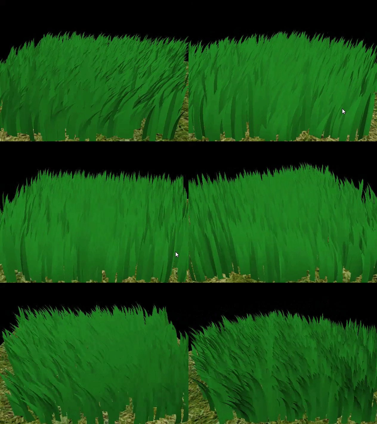 Consider the scenario in which the front face direction of the grass blade is perpendicular to the view vector. Since our grass blades
won't have width, we will end up trying to render parts of the grass that are actually smaller than the size of a pixel. This could
lead to aliasing artifacts.
In order to remedy this, we can cull these blades! Simply do a dot product test to see if the view vector and front face direction of
the blade are perpendicular. For this we use a threshold value of 0.8 to cull.
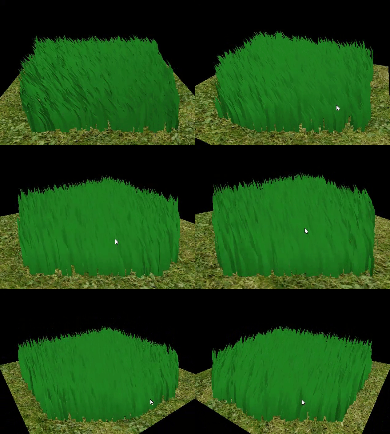 We also want to cull blades that are outside of the view-frustum, considering they won't show up in the frame anyway. To determine if
a grass blade is in the view-frustum, we want to compare the visibility of three points:
 v0, v2, and m, where m = (1/4)v0 * (1/2)v1 * (1/4)v2.
Notice that we aren't using v1 for the visibility test. This is because the v1 is a Bezier guide that doesn't represent a position on the grass blade.
We instead use m to approximate the midpoint of our Bezier curve.
If all three points are outside of the view-frustum, we will cull the grass blade. The paper uses a tolerance value for this test so that we are culling blades a little more conservatively. This can help with cases in which the Bezier curve is technically not visible, but we might be able to see the blade if we consider its width.
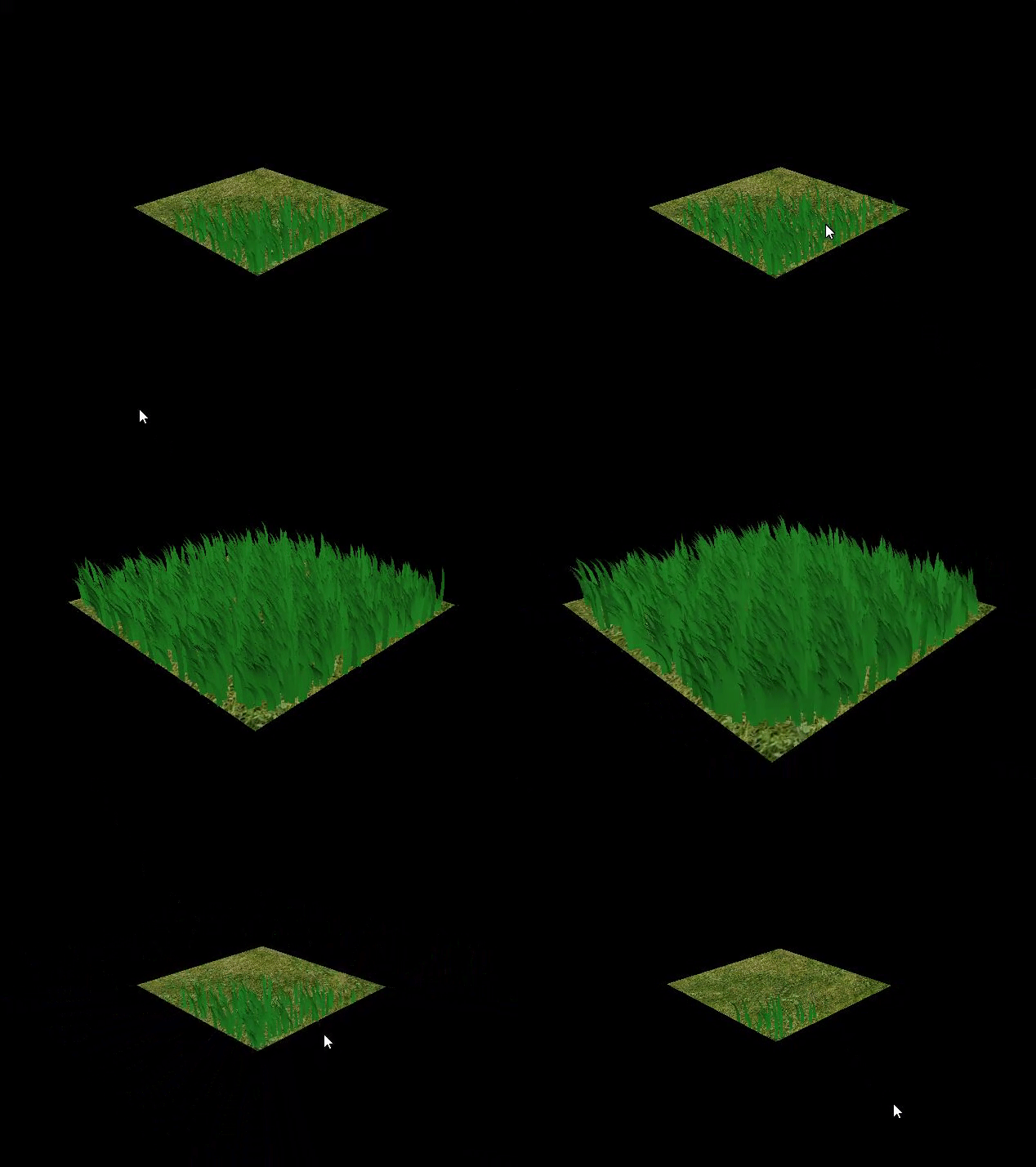 Similarly to orientation culling, we can end up with grass blades that at large distances are smaller than the size of a pixel. This could lead to additional
artifacts in our renders. In this case, we can cull grass blades as a function of their distance from the camera.
We define two parameters here.
- A max distance afterwhich all grass blades will be culled.
- A number of buckets to place grass blades between the camera and max distance into.
The grass blades in the bucket closest to the camera are kept while an increasing number of grass blades are culled with each farther bucket.
In this project, we pass in each Bezier curve as a single patch to be processed by your grass graphics pipeline. We tessellate this patch into a quad with a quadratic shape
In the tessellation control shader, we set the base level of inner and outer tessellation for when the blades are at MAX_DISTANCE to be 2.0 and we set the highest level of tessellation to be 6.0 when the blades are at distance 0 and interpolate between them.
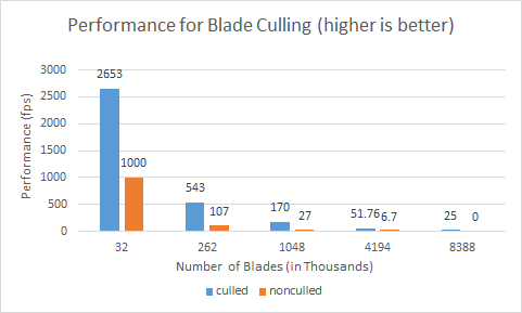
The performance we got for blade culling far outshined the performance we got for non-culling, despite having to do much more work in the compute shader. Without culling the blade count we were barely even able to render 4 million blades and we encountered substantial physics bugs on 8 million. As for the approach with culling, we were able to get a stable 25fps on 8 million blades and we hit a mak of 32 million blades (data point not shown).
The reason that culling improves performance so substantially here is the avoidance of entire extra pipeline calls. Despite spending much longer amount of time in the compute shader, that time is made up for by that blade never entering the grass blade render pass.
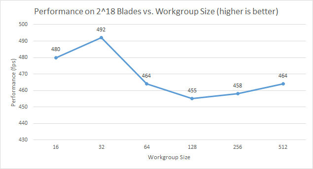
The optimal workgroup size, as we expected, was 32. The other workgoup sizes gave similar performance, but I believe 32 won out because it is the traditional size of a warp on NVIDIA hardware and so it was likely the GPU was easily able to handle scheduling logical blocks of 32 threads each.
The following resources were very useful in the creation of this project
