A New Context-Aware Details Injection Fidelity with Adaptive Coefficients Estimation for Variational Pansharpening [Matlab Code]
Homepage: https://liangjiandeng.github.io/
- Directly run:
demo_Pleiades_test.mfor a Pleiades example - Directly run:
demo_WV3_test.mfor a WV3 example
@ARTICLE{xiao2022tgrs,
author={J.-L. Xiao, T.-Z. Huang, L.-J. Deng, Z.-C. Wu, and G. Vivone},
booktitle={IEEE Trans. Geosci. Remote Sens.},
title={A New Context-Aware Details Injection Fidelity with Adaptive Coefficients Estimation for Variational Pansharpening},
year={2022},
pages={DOI: 10.1109/TGRS.2022.3154480},
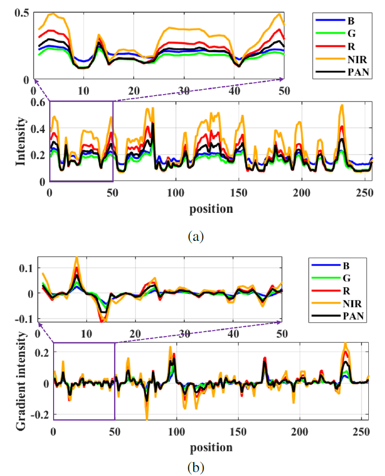
}Motivation: Fig. 1. (a) Plot of the intensity for both the PAN image and the HRMS data randomly choosing a row of the image; (b) Plot of the gradient intensity for both the PAN image and the HRMS data considering blue (B), green (G), red (R), and near-infrared (NIR) bands for the same row as in (a). It is worth to be remarked that the behavior of PAN and HRMS images is more similar in the gradient domain than in the intensity domain.
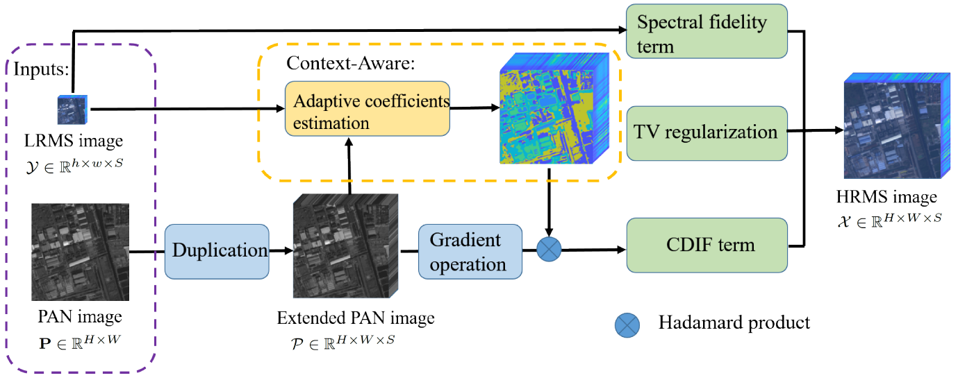
Overall Framework: The framework of our model. The details of our framework can be found in Sect. III.
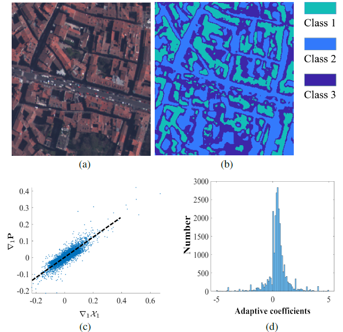
Fidelity: Fig. 4. (a) A close-up of the HRMS image of the Ple´iades dataset; (b) Context-aware regions extracted from (a); (c) Scatter plot of ∇1X1 and ∇1P for pixels belonging to Class 1 in (b); (d) A histogram of ∇1X1 � ∇1P for pixels belonging to Class 1 in (b). It is worth to be remarked that the distribution of ∇1X1 and ∇1P is well described by a directly proportional function, i.e., the black dotted line in (c). For other regions and bands, there is a similar directly proportional relationship between HRMS and PAN images in the gradient domain. Thus, the values of ∇X�∇P are approximately the same inside each region and for each band.
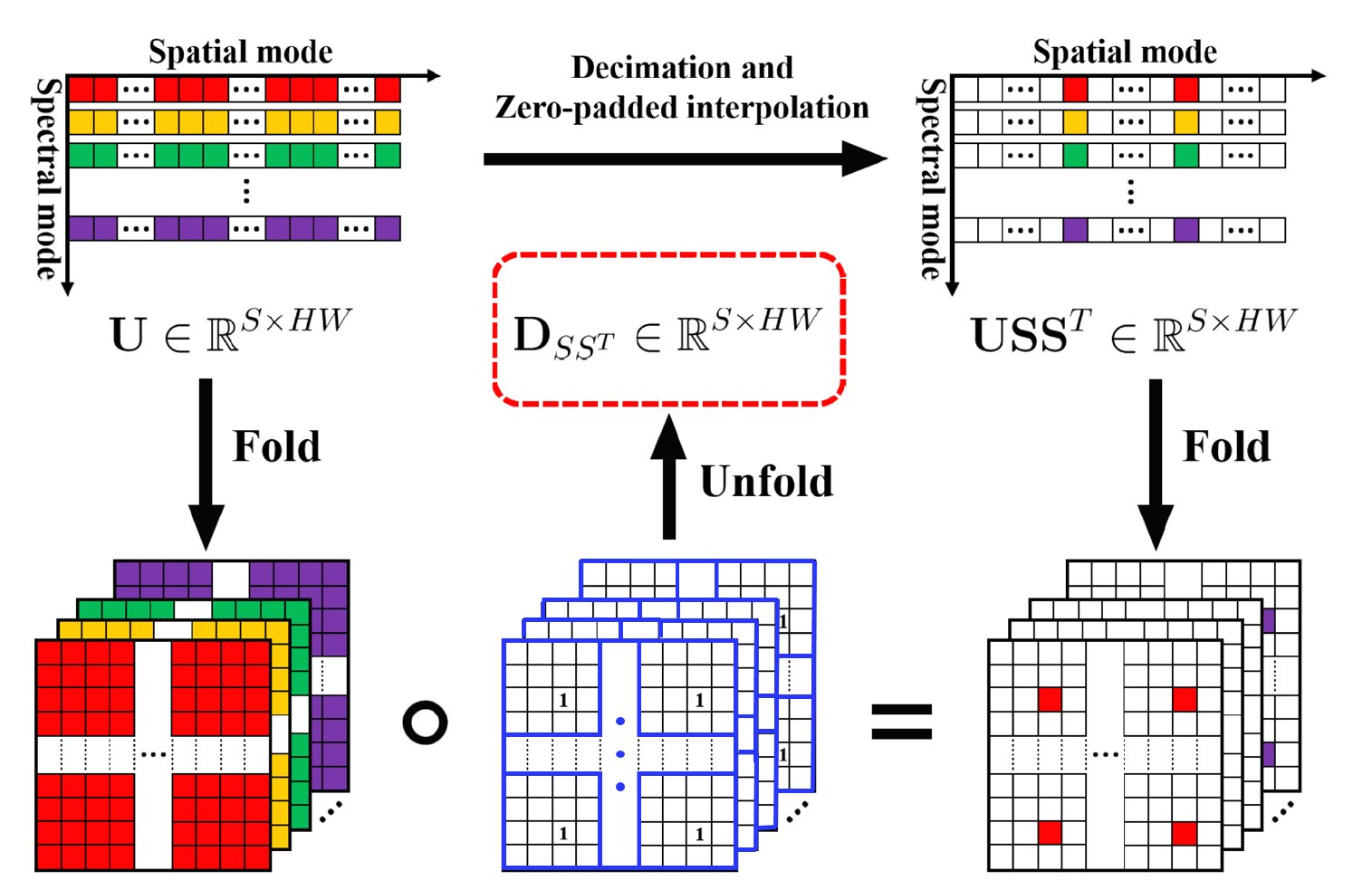
Handling the decimation operation: Fig. 5. The graphic representation of (22) for a scale ratio equal to 4. The white squares with a blank content indicate zero values. The first row shows the processing from U to USST, which is equal to an element-wise multiplication between DSST and U, i.e., the second row. It is worth noting that DSST is produced from sparse matrices (i.e., the blue squares), whose entries are 1 only in one position [44].
Final Model:
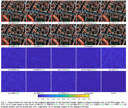
Visual Results: Fig. 6. Fusion results with close-ups for the compared approaches on the four-band Ple´iades dataset at reduced resolution (size of the PAN image: 256 × 256). . (a)-(j) Visual results in true colors of PRACS [9], RBDSD [49], C-GLP [59], GLP-Reg-FS [43], LGC [37], HQBP [60], PNN [19], TPNN [61], the proposed method, and the ground-truth (GT), respectively. (k)-(t) Residual images for the displayed red band.
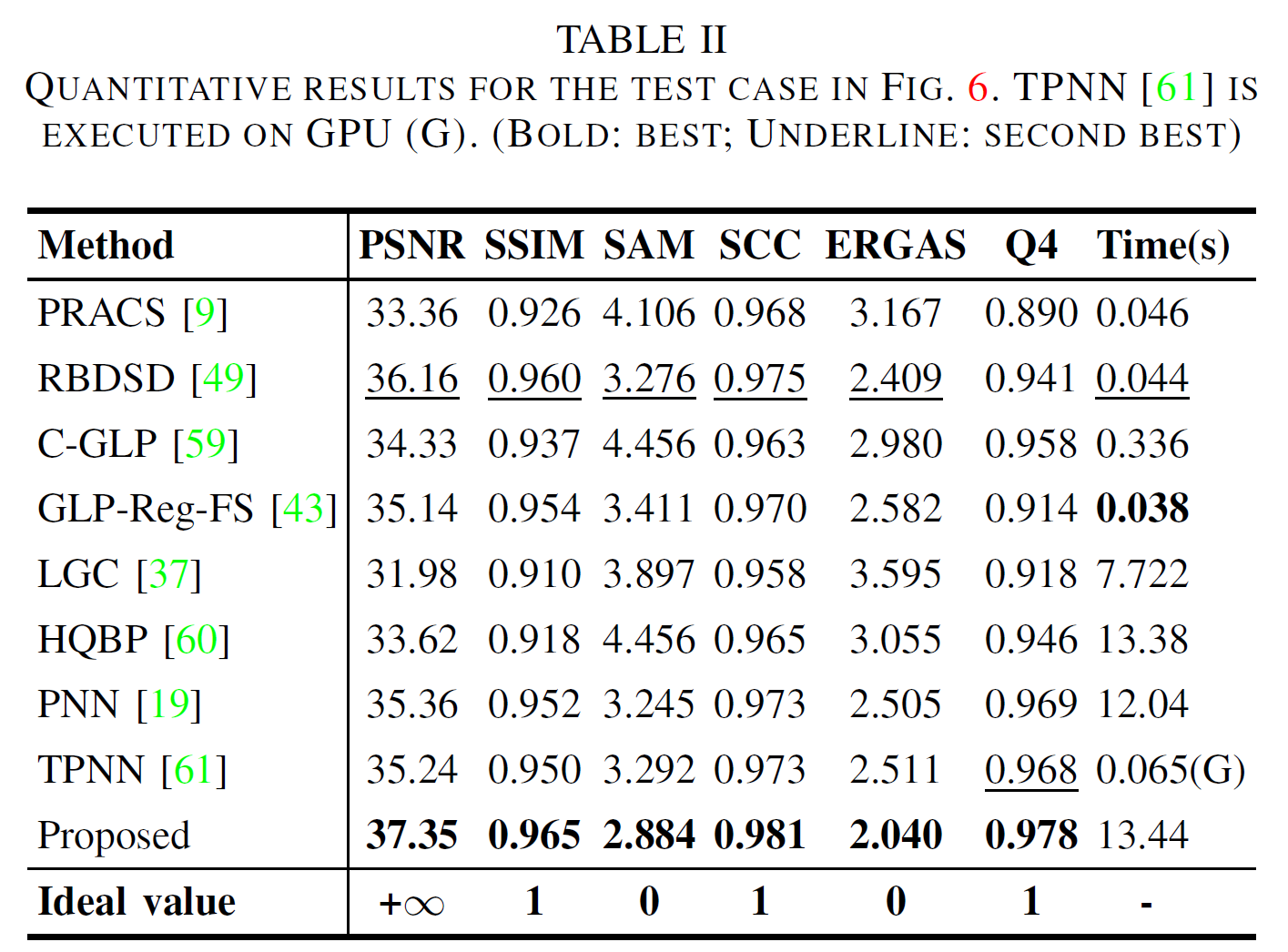
Quantitative Results: The quantitative results of Fig. 6.
