| title | output |
|---|---|
ExpressAnalystR |
html_document |
- Description
- Installation
- Tips for using the ExpressAnalystR package
- Examples
- 1. Starting from a gene expression matrix
- 1.1 Load ExpressAnalystR library and initialize R objects
- 1.2 Read data table
- 1.3 Annotate gene IDs to Entrez
- 1.4 Perform data filtering and normalization
- 1.5 Prepare differential expression (DE) analysis
- 1.6 Perform DE analysis and check DE results
- 1.7 Visualize gene expression pattern of individual gene
- 2. Starting from three datasets for meta-analysis
- 1. Starting from a gene expression matrix
ExpressAnalystR is the underlying R package synchronized with ExpressAnalyst web server. It is designed for statistical analysis, enrichment analysis and visual analytics of single and multiple gene expression data, both matrix and gene list. The R package is composed of R functions necessary for the web-server to perform data annotation, normalization, differential expression and meta-analysis.
Following installation and loading of ExpressAnalystR, users will be able to reproduce web server results from their local computers using the R command history downloaded from ExpressAnalystR. Running the R functions will allow more flexibility and reproducibility.
Note - ExpressAnalystR is still under development - we cannot guarantee full functionality
To use ExpressAnalystR, make sure your R version is >4.0.3 and install all package dependencies. Ensure that you are able to download packages from Bioconductor. To install package dependencies, use the pacman R package. Note that some of these packages may require additional library dependencies that need to be installed prior to their own successful installation.
install.packages("pacman")

library(pacman)

pacman::p_load(igraph, RColorBrewer, qs, rjson, RSQLite)
ExpressAnalystR is freely available from GitHub. The package documentation, including the vignettes for each module and user manual is available within the downloaded R package file. If all package dependencies were installed, you will be able to install the ExpressAnalystR.
Install the package directly from github using the devtools package. Open R and enter:
# Step 1: Install devtools
install.packages('devtools')
library(devtools)

# Step 2: Install ExpressAnalystR WITHOUT documentation
devtools::install_github("xia-lab/ExpressAnalystR", build = TRUE, build_opts = c("--no-resave-data", "--no-manual", "--no-build-vignettes"))

# Step 2: Install ExpressAnalystR WITH documentation
devtools::install_github("xia-lab/ExpressAnalystR", build = TRUE, build_opts = c("--no-resave-data", "--no-manual"), build_vignettes = TRUE)
- The first function that you will use in every module is the
Init.Datafunction, which initiates R objects that stores user's data, parameters for further processing and analysis. - The ExpressAnalystR package will output data files/tables/analysis/networks outputs in your current working directory.
- Every function must be executed in sequence as it is shown on the R Command history, please do not skip any commands as this can result in errors downstream.
- Main functions in ExpressAnalystR are documented. Use the ?Function format to open its documentation. For instance, use
?ExpressAnalystR::ReadTabExpressionto find out more about this function. - It is recommended to set the working folder to an empty folder because numerous files will be generated through the process.
- R package is not useful for visual analytics as they are hosted on the website. It's mainly useful for statistical analysis (differential expression and meta-analysis).
- R package is derived from R scripts used for powering web server. The values returned are often not useful in the context of local usage. The results from R functions are saved in a format qs file named as the file name of original data table. For gene list, the format qs file is named "datalist1". use this function to access:
dataSet <- readDataset(fileName)
Before you start, please download the example dataset. It is a microarray gene expression data of a human breast-cancer cell line.
library(ExpressAnalystR)

#boolean FALSE indicates local mode (vs web mode);
Init.Data(FALSE);

# Set analysis type to single gene expression matrix
SetAnalType("onedata");
dataSets <- ReadTabExpressData("estrogen.txt");
For this step it is imortant to please select correct organism, data type (array or RNA-seq), id type and gene-level summary (mean, median, sum). For gene-level summary, microarray can use mean or median while RNA-seq needs to be sum.
dataSets <- PerformDataAnnot("estrogen.txt", "hsa", "array", "hgu95av2", "mean");
Take a look at the mapped dataset by reading the dataset's qs file using readDataset(fileName) function.
dataSet <- readDataset("estrogen.txt")
print(head(dataSet$data.anot[c(1:5),]))
Check diagnostics plots to look at overall data distribution, sample separation.
PlotDataBox("estrogen.txt", "qc_boxplot_", 72, "png");
PlotDataPCA("estrogen.txt", "qc_pca_", 72, "png");
Check your working directory for png images named qc_boxplot_dpi72.png and qc_pca_dpi72.png, open them.
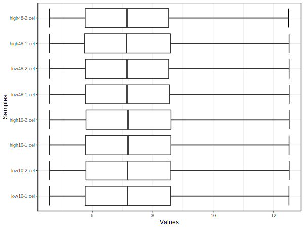
Box plot shows that the expression distribution of samples are between around -4 to 12.5. This shows that the data has already been normalized.
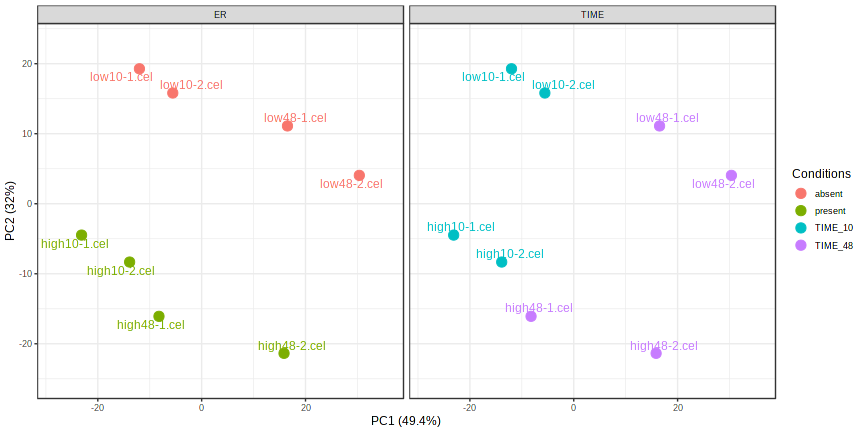
No normalization need to be performed, PCA plot from previous step shows that the dataset is already normalized. Filter by variance (lower 15% removed) Filter by relative abundance (lower 4 percentile of average expression signal) Filter by count not applied (only for RNASeq data) Filter unannotated genes TRUE
dataSets <- PerformExpressNormalization("estrogen.txt", "none", 15, 4, 0);
Selected metadata of interest, in this case we are interested in investigating the effect of presence of Estrogen Receptor (ER) vs absence. We are not setting secondary factor and blocking factor. After selecting metadata, compute design matrix and select DE analysis algorithm by running SetupDesignMatrix function. For microarray data, only limma can be used.
dataSets <- SetSelectedMetaInfo("estrogen.txt","ER", "NA", F);
dataSets <- SetupDesignMatrix("estrogen.txt", "limma");
Fold change is log2 transformed. Adjusted P-value using False Discovery Rate (FDR) method.
dataSets <- PerformDEAnal("estrogen.txt", "custom", "absent vs. present", "NA", "intonly");
dataSet <- readDataset("estrogen.txt");
print(head(dataSet$comp.res));
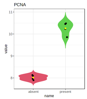
PlotSelectedGene("estrogen.txt","5111");
Check the resulting png image (Gene_5111.png) in your working directory.
Before you start, please download the example datasets into your working directory E-GEOD-25713, E-GEOD-59276.txt, GSE69588.txt. These three testing datasets (containing subset of 5000 genes) are from a meta-analysis of helminth infections in mouse liver.
library(ExpressAnalystR)

#boolean FALSE indicates local mode (vs web mode);
Init.Data(FALSE);

# Set analysis type to meta-analysis
SetAnalType("metadata");
#Read dataset text file
dataSets <- ReadOmicsData("E-GEOD-25713.txt");
dataSets <- SanityCheckData("E-GEOD-25713.txt");

#Map gene id to entrez id
dataSets <- AnnotateGeneData("E-GEOD-25713.txt", "mmu", "entrez");
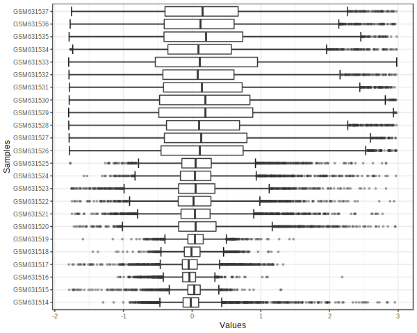
Visually inspect dataset using box plot (qc_boxplot_0_dpi72.png) and pca plot (qc_pca_0_dpi72.png).
PlotDataProfile("E-GEOD-25713.txt", "raw", "qc_boxplot_0_", "qc_pca_0_");
#Remove variables with more than 50% missing data
dataSets <- RemoveMissingPercent("E-GEOD-25713.txt", 0.5);

#Replace missing value with minimum values across dataset
dataSets <- ImputeMissingVar("E-GEOD-25713.txt", "min");

#Replace missing value with minimum values across dataset
dataSets <- NormalizingDataMeta("E-GEOD-25713.txt", "NA");
dataSets <- PerformDEAnalMeta("E-GEOD-25713.txt", "limma", "CLASS", 0.05, 0.0);

#read and process the other two datasets
dataSets <- ReadOmicsData("E-GEOD-59276.txt");
dataSets <- SanityCheckData("E-GEOD-59276.txt");
dataSets <- AnnotateGeneData("E-GEOD-59276.txt", "mmu", "entrez");
dataSets <- RemoveMissingPercent("E-GEOD-59276.txt", 0.5)
dataSets <- ImputeMissingVar("E-GEOD-59276.txt", "min")
dataSets <- NormalizingDataMeta("E-GEOD-59276.txt", "NA");
dataSets <- PerformDEAnalMeta("E-GEOD-59276.txt", "limma", "CLASS", 0.05, 0.0);

dataSets <- ReadOmicsData("GSE69588.txt");
dataSets <- SanityCheckData("GSE69588.txt");
dataSets <- AnnotateGeneData("GSE69588.txt", "mmu", "entrez");
dataSets <- RemoveMissingPercent("GSE69588.txt", 0.5)
dataSets <- ImputeMissingVar("GSE69588.txt", "min")
dataSets <- NormalizingDataMeta("GSE69588.txt", "NA");
dataSets <- PerformDEAnalMeta("GSE69588.txt", "limma", "CLASS", 0.05, 0.0);
CheckMetaDataIntegrity();
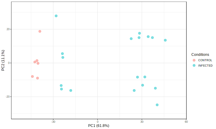
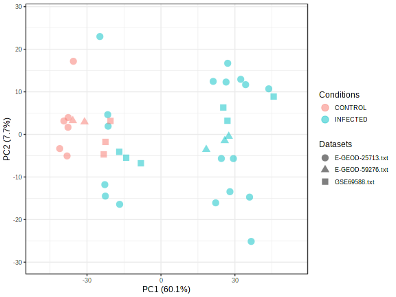
PlotMetaPCA("qc_meta_pca_","72", "png", "");

There is clear signs of batch effect. The samples from same dataset are largely clustered together. To remove the batch effect, we need to run comBat batch correction algorithm
#Apply batch effect correction
PerformBatchCorrection();

#Check the result
PlotMetaPCA("qc_meta_pca_afterBatch_","72", "png", "");
Here is the result after batch correction.
analSet <- PerformPvalCombination("fisher", 0.05)
analSet <- readSet(analSet, "analSet");
print(head(analSet$meta.mat));
       CombinedTstat CombinedPval
16854         89.093   2.7728e-14
246256        99.964   2.7728e-14
105855        94.751   2.7728e-14
19241        105.030   2.7728e-14
319169        94.339   2.7728e-14
16819        100.880   2.7728e-14
For a more detailed table containing additionally log fold change and p-values of features for individual dataset, please check this csv file meta_sig_genes_metap.csv, it is also generated in your working directory.
