In this project, I used deep neural networks and three classic convolutional neural network architectures(LeNet, AlexNet and GoogLeNet) to classify traffic signs. I will train and validate a model so it can classify traffic sign images using the German Traffic Sign Dataset. After the model is trained, I will then try out my model on images of German traffic signs that I find on the web.
- Load and explore the data set.
- Realize LeNet architecture and use
ReLu,mini-batch gradient descentanddropout. - Realize AlexNet and make some modifications, use
learning rate decay,Adam optimizationandL2 regulization. - Use GoogLeNet to classify traffic signs and make some modifications, use
inceptionandoverlapping poolingandaverage pooling. - Analyze the softmax probabilities of the new images
- Summarize the results
python3.5
matplotlib (2.1.1)
opencv-python (3.3.1.11)
numpy (1.13.3)
tensorflow-gpu (1.4.1)
sklearn (0.19.1)
Download the data set. This is a pickled dataset in which the images are already resized to 32x32. It contains a training, validation and test set.
I used the numpy library to calculate summary statistics of the traffic signs data set:
- The size of training set is: 34799
- The size of the validation set is: 4410
- The size of test set is: 12630
- The shape of a traffic sign image is: (32, 32 ,3)
- The number of unique classes/labels in the data set is: 43
Here is an exploratory visualization of the training data set.
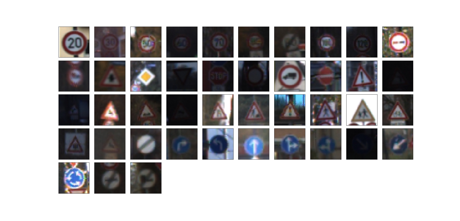
The distribution of training, validation and testing set is showing in the following bar charts.

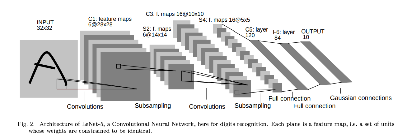
The LeNet model is proposed by Yann LeCun in 1998, it is the most classific cnn model for image recognition, its architecture is as following:
In the LeNet architecture I realized for traffic signs recognition, three tricks as used as follows:
- 1 ReLu
ReLu nonlinear function is used as the activation function after the convolutional layer. More information about ReLu and other activation functions can be find at Lecture 6 | Training Neural Networks I. - 2 Mini-batch gradient descent
Mini-batch gradient descent is the combine of batch gradient descent and stochastic gradient descent, it is based on the statistics to estimate the average of gradient of all the training data by a batch of selected samples. - 3 Dropout
Dropout is a regularization technique for reducing overfitting in neural networks by preventing complex co-adaptations on training data. It is proposed in the paper Dropout: A Simple Way to Prevent Neural Networks from Overfitting. It is usually after fully connected layers. Awkwardly, there is a very small problem that LeNet will not overfitting to trainging set sometimes. Thus the dropout will not play a big role or even make the model worse for simple like LeNet. And the training set error maybe be higher than validation set error while training.
My LeNet consists of the following layers:
| Layer | Description | Input | Output |
|---|---|---|---|
| Convolution | kernel: 5x5; stride:1x1; padding: valid | 32x32x3 | 28x28x6 |
| Max pooling | kernel: 2x2; stride:2x2; | 28x28x6 | 14x14x6 |
| Convolution | kernel: 5x5; stride:1x1; padding: valid | 14x14x6 | 10x10x16 |
| Max pooling | kernel: 2x2; stride:2x2; | 10x10x16 | 5x5x16 |
| Flatten | Input 5x5x16 -> Output 400 | 5x5x16 | 400 |
| Fully connected | connect every neurel with next layer | 400 | 120 |
| Fully connected | connect every neurel with next layer | 120 | 80 |
| Fully connected | output 43 probabilities for each lablel | 80 | 43 |
I have turned the following three hyperparameters to train my model.
LEARNING_RATE = 1e-2
EPOCHS = 50
BATCH_SIZE = 128
It takes about 2 minutes to train the model on GetForce 750 ti.
The results are:
- accuracy of training set: 96.6%
- accuracy of validation set: 92.0%
- accuracy of test set: 89.7%
We can see that the model is overfitting to the training data and the accuracy on validation set is a little lower than on training set. The LeNet model is efficient and simple, many cnn architectures are inspired by it, like AlexNet.
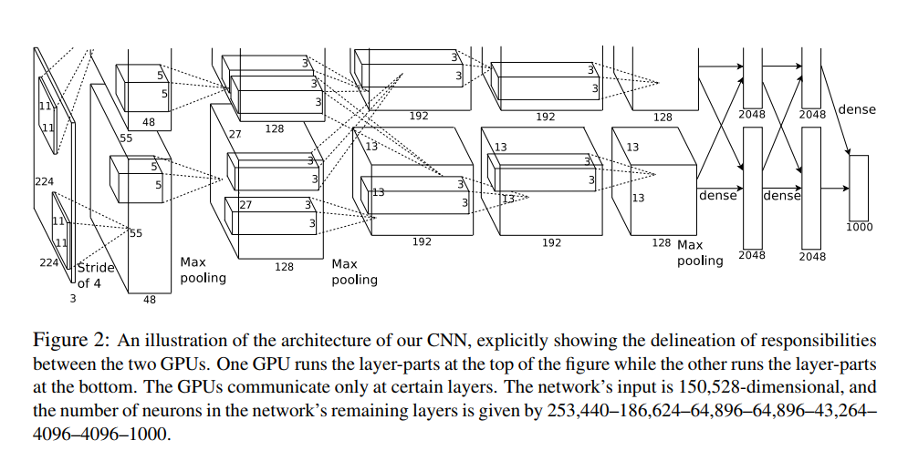
AlexNet is the first popularized CNN architecture in computer vision developed by Alex Krizhevsky, Geoffrey Hinton, and Ilya Sutskever. It is the champion of ImageNet ILSVRC challenge in 2012 and significantly outperformed the second runner-up. The AlexNet has a similar architecture with LeNet, but it is deeper and bigger.
Cause the input dimension and output dimension of traffic signs recognition on GTRSB is 32x32x3 and 43, which is different from the original dimension of AlexNet, so I made some change to fit the requirement. And the architecture I realized for recognizing traffic signs as the following table:
| Layer | Description | Input | Output |
|---|---|---|---|
| Convolution | kernel: 5x5; stride:1x1; padding: valid | 32x32x3 | 28x28x9 |
| Max pooling | kernel: 2x2; stride:2x2; | 28x28x9 | 14x14x9 |
| Convolution | kernel: 3x3; stride:1x1; padding: valid | 14x14x9 | 12x12x32 |
| Max pooling | kernel: 2x2; stride:2x2; | 12x12x32 | 6x6x32 |
| Convolution | kernel: 3x3; stride:1x1; padding: same | 6x6x32 | 6x6x48 |
| Convolution | kernel: 3x3; stride:1x1; padding: same | 6x6x48 | 6x6x64 |
| Convolution | kernel: 3x3; stride:1x1; padding: same | 6x6x64 | 6x6x96 |
| Max pooling | kernel: 2x2; stride:2x2; | 6x6x96 | 3x3x96 |
| Flatten | Input 3x3x96 -> Output 864 | 3x3x96 | 864 |
| Fully connected | connect every neurel with next layer | 864 | 400 |
| Fully connected | connect every neurel with next layer | 400 | 160 |
| Fully connected | output 43 probabilities for each lablel | 160 | 43 |
Apart from this, I have used following methods to make the model work better:
- Learning rate decay
In training deep networks, when the learning rate is large, the system contains too much kinetic energy and the parameter vector bounces around chaotically, ubable to settle down into deeper; when the learning rate is small, you will be wasting computation bouncing around chaotically with little improvement for a long time. If the learning rate can decay from large to small while training, the network will move fast at the begining and improve little by little in the end. There are three commonly used types of method: step dacay, exponential decay and 1/t decay, more information can be found here and here. Cause I use tensorflow to realize AlexNet and exponential dacay are used for learning decay, so I choose it as my method, its usage can be find here is used to decay learning rate. Maybe it is not a good method, since there is tow more hyper parameters (decay_step and decay_rate) to tune. - Adam optimization
Adam is a popular optimization recently proposed by Diederik P. Kingma and Jimmy Ba, like previous proposed Adagrad and RMSprop, it is a kind of adaptive learning rate method. With Adam, we don't have to use learning rate decay and tune three parameters for perfect learning rate. It is fabilous, so I will use it in most of times. After adapting Adam, the accuracy for training set, validation set and testing set are 99.9%, 96.9% and 94.2% respectively. The model is a little overfitting to training set, so some regularization methods are used to reduce it. - L2 regulization
L2 regulization is used to reduce overfitting by adding regulization loss to loss function, it is based on the assume that the bigger regulization loss is the more complex the model is. It is well known that complex model is more easily overfit to training set, thus, through reducing regulization loss to make the model simpler. The regulization loss is the sum of L2 norm of weights for each layer multiple regulization parameterlambdain most cases,lambdais a small positive number that controls the regulization degree. Tensorflow documetn for how to use l2 regulization can be find here.
I have turned the following three hyperparameters to train my model.
- LEARNING_RATE = 5e-4
- EPOCHS = 30
- BATCH_SIZE = 128
- keep_prop = 0.5
- LAMBDA = 1e-5
The results are:
- accuracy of training set: 100.0%
- accuracy of validation set: 96.0%
- accuracy of test set: 94.6%
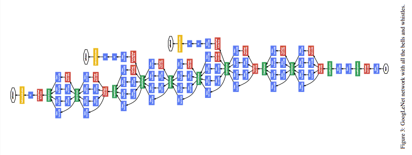
GoogLeNet was the winner of the ILSVRC 2014, it main contribution was the development of Inception Module that dramatically reduced the number of parameters in the network.
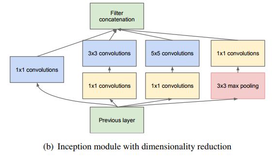
Additionally, this paper uses Average Pooling instead of Fully connected layer at the top of the ConvNet, eliminating a large amount of parameters that do not seem to matter much. The overall architecture of GoogLeNet is as the following table.
The original architecture of GoogLeNet is a little hard to train by my GPU, so I choose to reduce the number of layers from 22 to 14, the details of network is showing in the following table.
| Type | Kernel/Stride | Output | Parameters |
|---|---|---|---|
| conv | 3x3/2x2 | 16x16x64 | 1,792 |
| inception(2a) | 16x16x256 | 137,072 | |
| inception(2b) | 16x16x480 | 388,736 | |
| max pool | 3x3/2x2 | 7x7x480 | |
| inception(3a) | 7x7x512 | 433,792 | |
| inception(3a) | 7x7x512 | 449,160 | |
| max pool | 3x3/2x2 | 3x3x512 | |
| inception(4a) | 3x3x832 | 859,136 | |
| inception(4a) | 3x3x1024 | 1,444,080 | |
| avg pool | 3x3/1x1 | 1x1x1024 | |
| flatten | 864 | 1024 | |
| full | 43 | 43 | 44,032 |
Some details for this architecture is as following:
- Inception Module
The inception module is the core of this architecture, it is driven by two disadvantage of previous architecture: a large amount of parameters which lead to overfitting and dramatically use of computational resources. It's navie implement doesn't have 1x1 conv before/after 3x3 conv, 5x5 conv and max pooling layer. The reason why adding 1x1 convolutional layer is that it can reduce the depth of the output from previous layer, therefore, the amount of operations can be significantly reduced. More details can be found in Going deeper with convolutions. Since max pooling will reduce the shape of input feature map, so I realize it by padding with zeros and another implement can look here. - Overlapping pooling
The normal pooling operation is with kernel size = 2 and stride = 2, and the overlapping pooling means kernel size > stride, like kernel size = 3 and stride = 2, thus there will be overlapping fields. According to Traffic Sign Recognition with Multi-Scale Convolutional Networks, overlapping pooling can slightly reduce the error rates compared to non-overlapping and make the model more difficult to overfit.
I have turned the following three hyperparameters to train my model.
- LEARNING_RATE = 5e-4
- EPOCHS = 35
- BATCH_SIZE = 128
- keep_prop = 0.5
The results are:
- accuracy of training set: 100.0%
- accuracy of validation set: 98.5%
- accuracy of test set: 98.1%
In this project, I use three classific CNN architecture to recognize traffic signs from GTSRB, they are LeNet, AlexNet and GoogLeNet. Since the original architecture may no be suit for images from GRSRB, so I made some changes to them. In addition, I use some methods and tricks to train the model, like mini-batch gradient descent, Adam optimization, L2 regularization, learning rate decay and so on. Finally, ten online traffic images are used to test my model, result shows that it work very well, all the ten signs are perfected recognized.
The German Traffic Sign Recognition Benchmark
Man vs. computer: Benchmarking machine learning algorithms for traffic sign recognition
Traffic Sign Recognition with Multi-Scale Convolutional Networks
The German Traffic Sign Recognition Benchmark: A multi-class classification competition
Gradient-Based Learning Applied to Document Recognition
ImageNet Classification with Deep Convolutional Neural Networks
Going deeper with convolutions
